Description:
Location: hypar/Examples/1D/Euler1D/LaxShockTube (This directory contains all the input files needed to run this case. If there is a Run.m, run it in MATLAB to quickly set up, run, and visualize the example).
Governing equations: 1D Euler equations (euler1d.h)
References:
- P.D. Lax, "Weak solutions of nonlinear hyperbolic
equations and their numerical computation," Comm. Pure App. Math., 7, 159 (1954).
- C. B. Laney, "Computational Gasdynamics", Cambridge University Press, 1998.
Domain: \(0 \le x \le 1.0\), "extrapolate" (_EXTRAPOLATE_) boundary conditions
Initial Solution:
- \( 0 \le x < 0.5\): \(\rho = 0.445, \rho u = 0.311, e = 8.928\)
- \( 0.5 \le x \le 1\): \(\rho = 0.5, \rho u = 0, e = 1.4275\)
Numerical Method:
Input files required:
solver.inp:
begin
ndims 1
nvars 3
size 201
iproc 2
ghost 3
n_iter 80
time_scheme rk
time_scheme_type 44
hyp_space_scheme weno5
hyp_interp_type characteristic
conservation_check yes
dt 0.001
screen_op_iter 10
file_op_iter 9999
op_file_format text
op_overwrite no
model euler1d
end
boundary.inp
2
extrapolate 0 1 0 0
extrapolate 0 -1 0 0
physics.inp
begin
gamma 1.4
upwinding rf-char
end
weno.inp (optional)
begin
mapped 1
borges 0
yc 0
no_limiting 0
epsilon 0.000001
p 2.0
rc 0.3
xi 0.001
end
To generate initial.inp, compile and run the following code in the run directory:
#include <stdio.h>
#include <stdlib.h>
#include <math.h>
#include <string.h>
int NI=101,ndims=1;
FILE *in;
char ip_file_type[50];
strcpy(ip_file_type,"ascii");
printf("Reading file \"solver.inp\"...\n");
in = fopen("solver.inp","r");
if (!in) printf("Error: Input file \"solver.inp\" not found. Default values will be used.\n");
else {
char word[500];
fscanf(in,"%s",word);
if (!strcmp(word, "begin")){
while (strcmp(word, "end")){
fscanf(in,"%s",word);
if (!strcmp(word, "ndims")) fscanf(in,"%d",&ndims);
else if (!strcmp(word, "size")) fscanf(in,"%d",&NI);
else if (!strcmp(word, "ip_file_type")) fscanf(in,"%s",ip_file_type);
}
} else printf("Error: Illegal format in solver.inp. Crash and burn!\n");
}
fclose(in);
if (ndims != 1) {
printf("ndims is not 1 in solver.inp. this code is to generate 1D initial conditions\n");
return(0);
}
printf("Grid:\t\t\t%d\n",NI);
int i;
double dx = 1.0 / ((double)(NI-1));
double *x, *rho,*rhou,*e;
x = (double*) calloc (NI, sizeof(double));
rho = (double*) calloc (NI, sizeof(double));
rhou = (double*) calloc (NI, sizeof(double));
e = (double*) calloc (NI, sizeof(double));
for (i = 0; i < NI; i++){
x[i] = i*dx;
double RHO,U,P;
if (x[i] < 0.5) {
rho[i] = 0.445;
rhou[i] = 0.311;
e[i] = 8.928;
} else {
rho[i] = 0.5;
rhou[i] = 0;
e[i] = 1.4275;
}
}
if (!strcmp(ip_file_type,"ascii")) {
FILE *out;
out = fopen("initial.inp","w");
for (i = 0; i < NI; i++) fprintf(out,"%lf ",x[i]);
fprintf(out,"\n");
for (i = 0; i < NI; i++) fprintf(out,"%lf ",rho[i]);
fprintf(out,"\n");
for (i = 0; i < NI; i++) fprintf(out,"%lf ",rhou[i]);
fprintf(out,"\n");
for (i = 0; i < NI; i++) fprintf(out,"%lf ",e[i]);
fprintf(out,"\n");
fclose(out);
} else if ((!strcmp(ip_file_type,"binary")) || (!strcmp(ip_file_type,"bin"))) {
printf("Error: Writing binary initial solution file not implemented. ");
printf("Please choose ip_file_type in solver.inp as \"ascii\".\n");
}
free(x);
free(rho);
free(rhou);
free(e);
return(0);
}
Output:
Note that iproc = 2 in solver.inp, so run this with 2 MPI ranks (or change iproc to 1). After running the code, there should be two solution output files op_00000.dat and op_00001.dat; the first one is the initial solution, and the latter is the final solution. Both these files are ASCII text (HyPar::op_file_format is set to text in solver.inp). In these files, the first column is grid index, the second column is x-coordinate, and the remaining columns are the solution components.
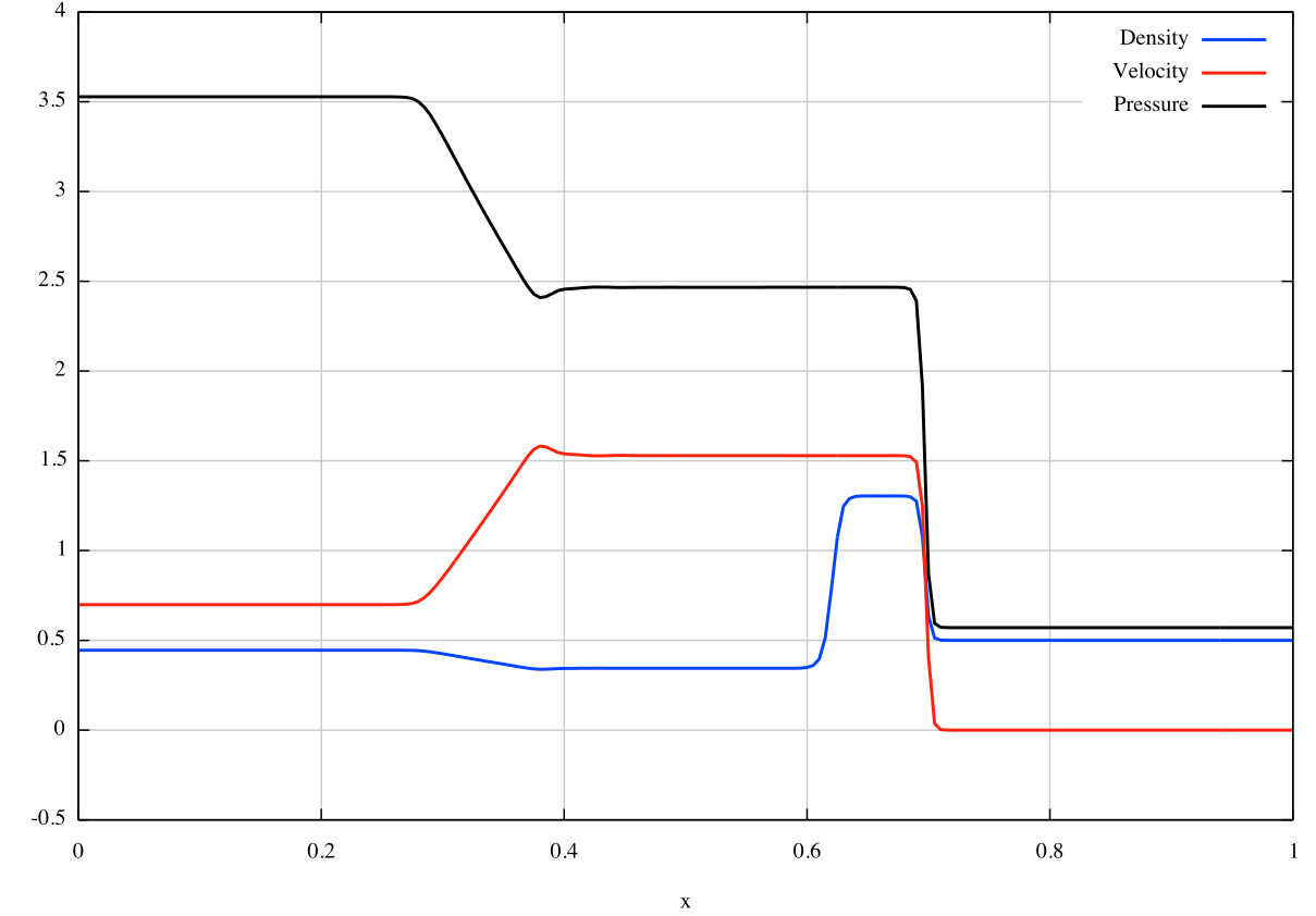
Final solution at t=0.08: The following figure is obtained by plotting op_00001.dat. Note that the output is in terms of the conserved variables, so they have to converted to the primitive variables (density, velocity, and pressure).
Since HyPar::ConservationCheck is set to yes in solver.inp, the code checks for conservation error and prints it to screen, as well as the file conservation.dat:
201 2 1.0000000000000000E-03 1.1102230246251565E-16 8.3266726846886741E-17 2.0556166428686216E-15
The numbers are: number of grid points (HyPar::dim_global), number of processors (MPIVariables::iproc), time step size (HyPar::dt), and conservation error (HyPar::ConservationError) for each component.
Expected screen output:
HyPar - Parallel (MPI) version with 2 processes
Compiled with PETSc time integration.
Reading solver inputs from file "solver.inp".
No. of dimensions : 1
No. of variables : 3
Domain size : 201
Processes along each dimension : 2
No. of ghosts pts : 3
No. of iter. : 80
Restart iteration : 0
Time integration scheme : rk (44)
Spatial discretization scheme (hyperbolic) : weno5
Split hyperbolic flux term? : no
Interpolation type for hyperbolic term : characteristic
Spatial discretization type (parabolic ) : nonconservative-1stage
Spatial discretization scheme (parabolic ) : 2
Time Step : 1.000000E-03
Check for conservation : yes
Screen output iterations : 10
File output iterations : 9999
Initial solution file type : ascii
Initial solution read mode : serial
Solution file write mode : serial
Solution file format : text
Overwrite solution file : no
Physical model : euler1d
Partitioning domain.
Allocating data arrays.
Reading array from ASCII file initial.inp (Serial mode).
Volume integral of the initial solution:
0: 4.7499999999999998E-01
1: 1.5550000000000000E-01
2: 5.1848875000000110E+00
Reading boundary conditions from "boundary.inp".
Boundary extrapolate: Along dimension 0 and face +1
Boundary extrapolate: Along dimension 0 and face -1
2 boundary condition(s) read.
Initializing solvers.
Reading WENO parameters from weno.inp.
Initializing physics. Model = "euler1d"
Reading physical model inputs from file "physics.inp".
Setting up time integration.
Solving in time (from 0 to 80 iterations)
Writing solution file op_00000.dat.
Iteration: 10 Time: 1.000E-02 Max CFL: 9.579E-01 Max Diff. No.: -1.000E+00 Norm: 1.4973E-01 Conservation loss: 8.5651E-16
Iteration: 20 Time: 2.000E-02 Max CFL: 9.526E-01 Max Diff. No.: -1.000E+00 Norm: 1.5211E-01 Conservation loss: 1.7148E-15
Iteration: 30 Time: 3.000E-02 Max CFL: 9.500E-01 Max Diff. No.: -1.000E+00 Norm: 1.5129E-01 Conservation loss: 1.3727E-15
Iteration: 40 Time: 4.000E-02 Max CFL: 9.492E-01 Max Diff. No.: -1.000E+00 Norm: 1.5139E-01 Conservation loss: 1.7166E-15
Iteration: 50 Time: 5.000E-02 Max CFL: 9.485E-01 Max Diff. No.: -1.000E+00 Norm: 1.5220E-01 Conservation loss: 1.7139E-15
Iteration: 60 Time: 6.000E-02 Max CFL: 9.480E-01 Max Diff. No.: -1.000E+00 Norm: 1.5340E-01 Conservation loss: 1.5467E-15
Iteration: 70 Time: 7.000E-02 Max CFL: 9.476E-01 Max Diff. No.: -1.000E+00 Norm: 1.5473E-01 Conservation loss: 1.8884E-15
Iteration: 80 Time: 8.000E-02 Max CFL: 9.472E-01 Max Diff. No.: -1.000E+00 Norm: 1.5596E-01 Conservation loss: 2.0603E-15
Writing solution file op_00001.dat.
Completed time integration (Final time: 0.080000).
Computed errors:
L1 Error : 0.0000000000000000E+00
L2 Error : 0.0000000000000000E+00
Linfinity Error : 0.0000000000000000E+00
Conservation Errors:
1.1102230246251565E-16
8.3266726846886741E-17
2.0556166428686216E-15
Solver runtime (in seconds): 1.1952400000000001E-01
Total runtime (in seconds): 1.2100000000000000E-01
Deallocating arrays.
Finished.