Initial solution: \(u\left(x,y,0\right) = u_0\left(x,y\right)= \sin\left(2\pi x\right)\cos\left(2\pi y\right)\)
Exact solution: \(u\left(x,y,t\right) = u_0\left(x-a_xt,y-a_yt\right)\).
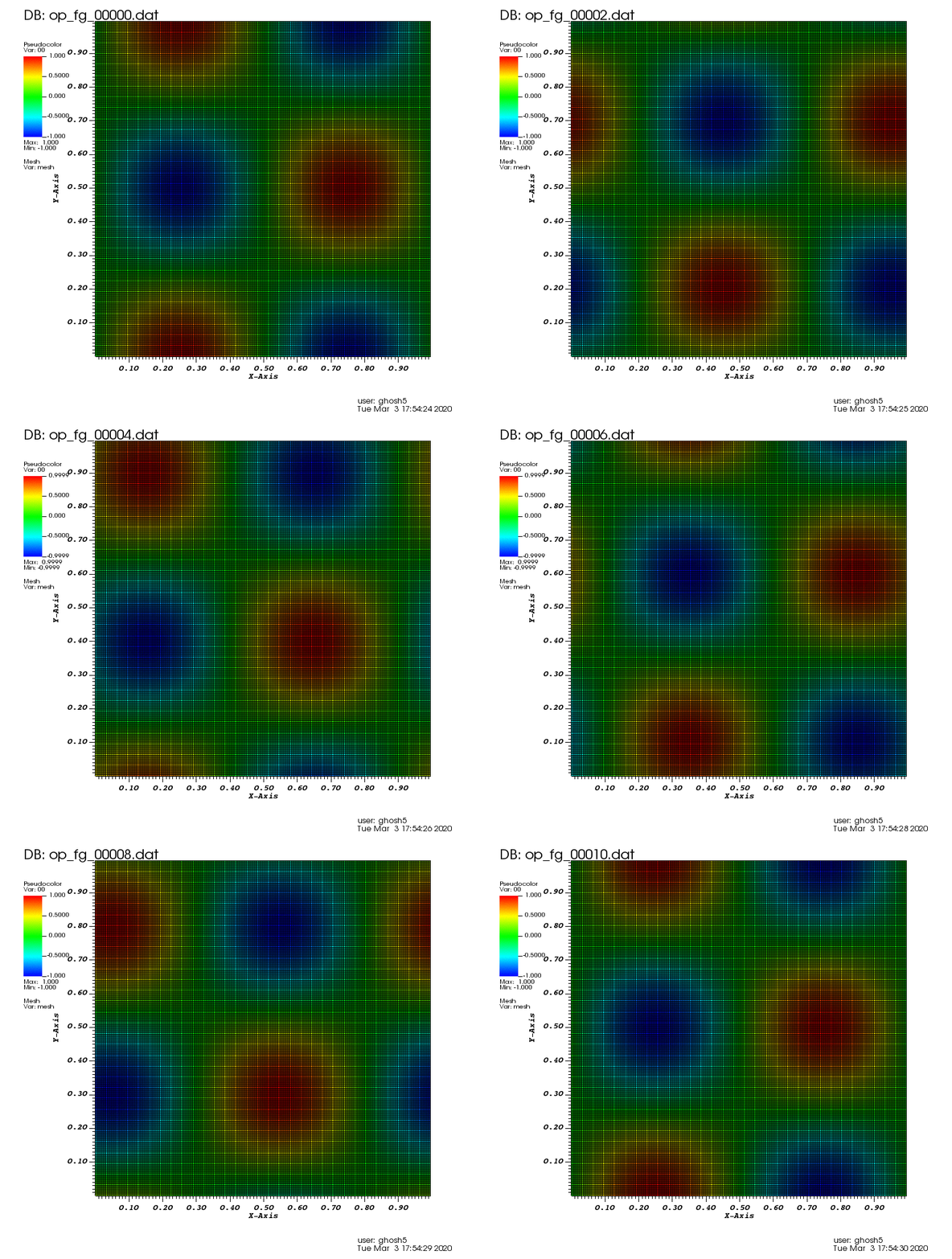
The following animation was generated from the full grid solution files that were computed by using the combination technique on the sparse grids:
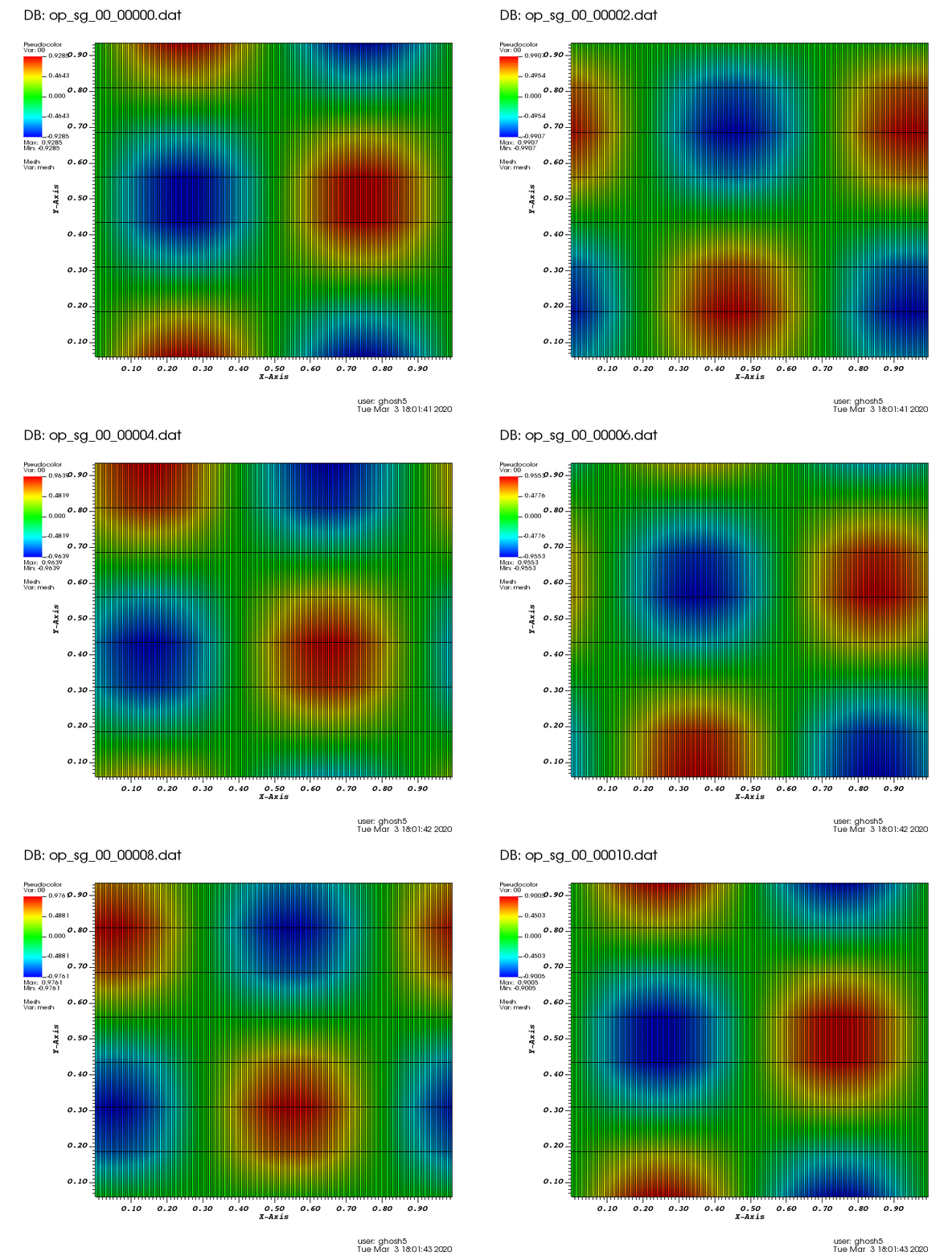
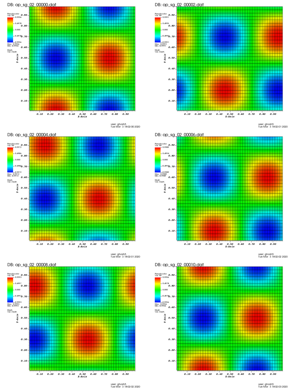
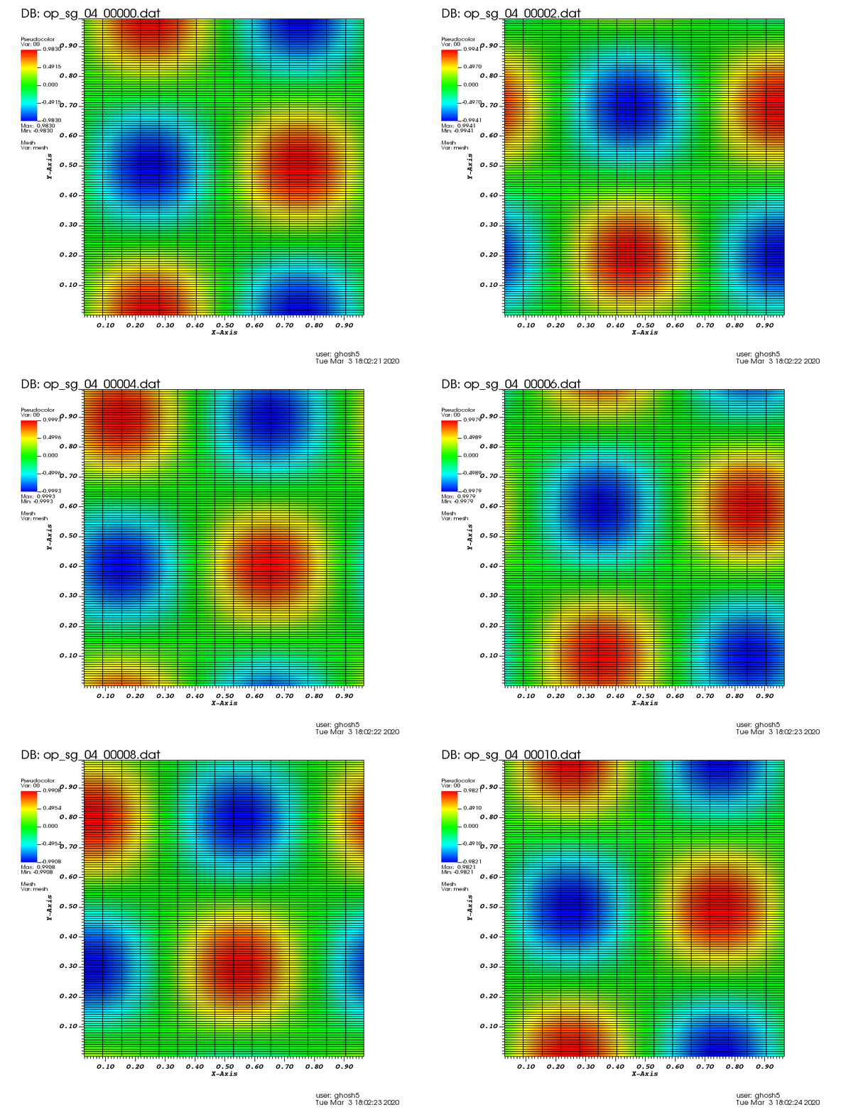
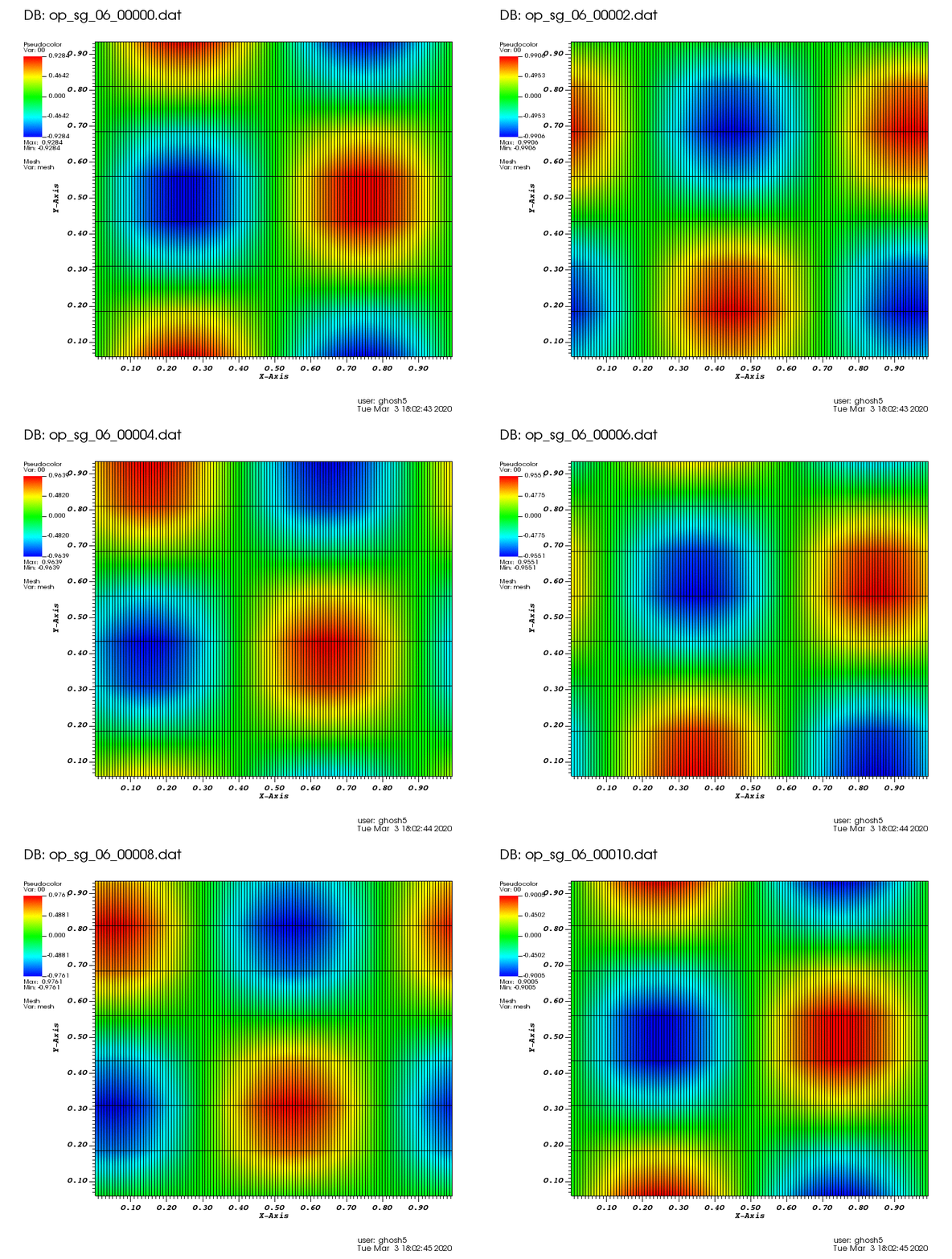
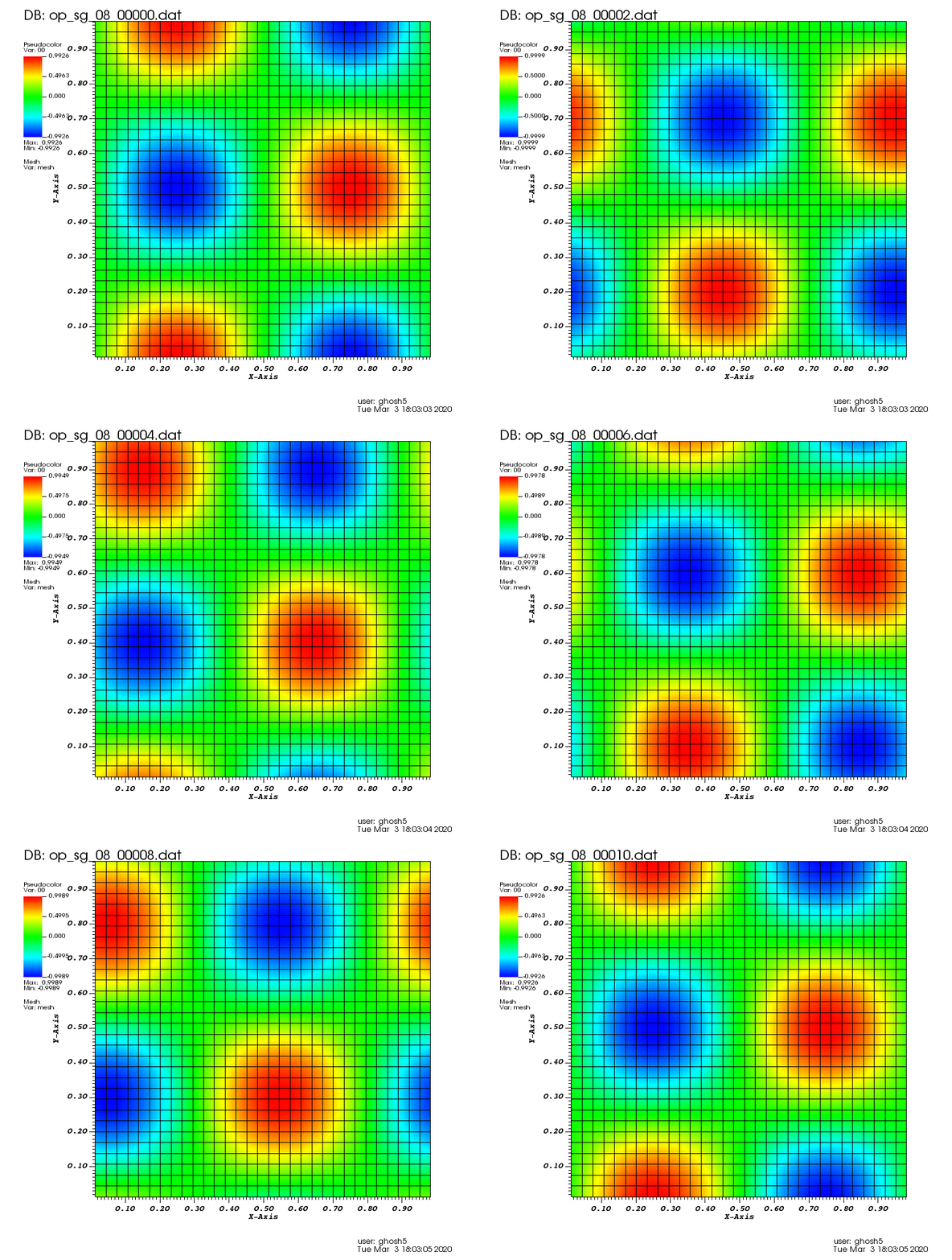
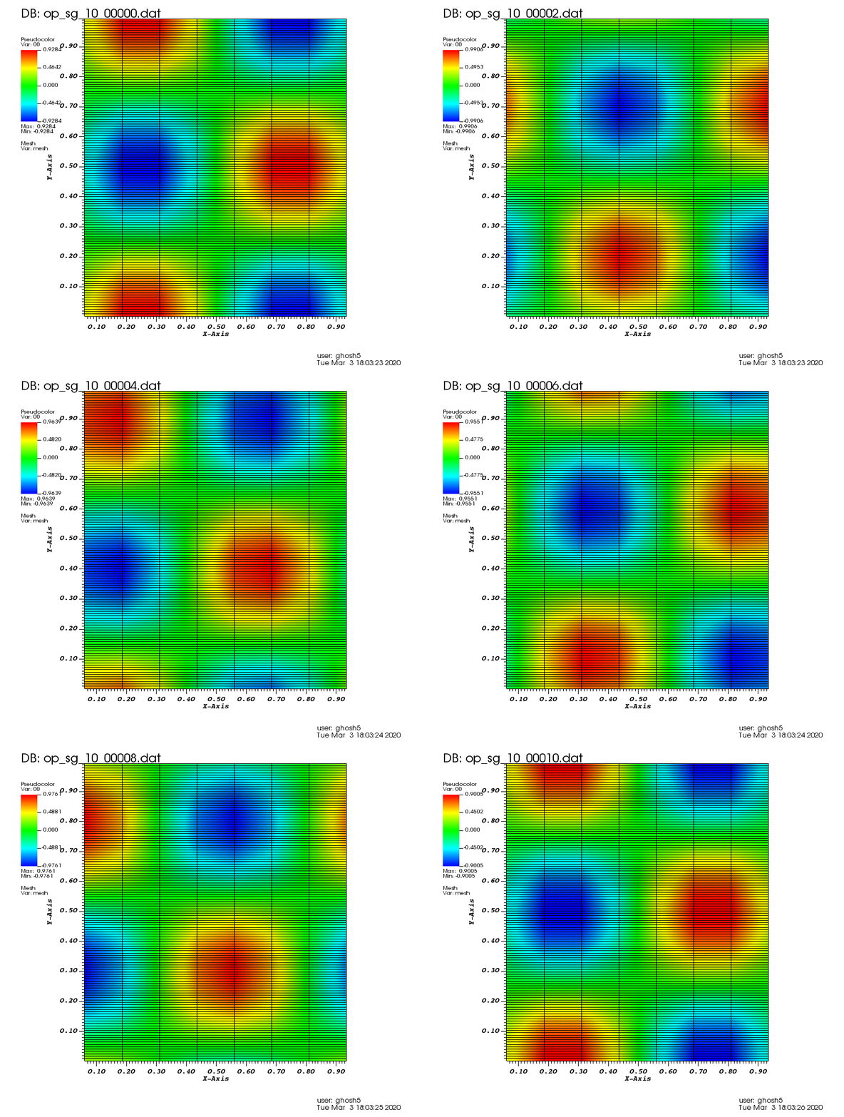
The following animations show the solution on some of the sparse grids in the combination technique. The simulation was actually carried out on these grids. Note the different grid sizes.
Since the exact solution is available at the final time, the numerical errors are calculated for the recombined full grid solution and reported on screen (see below) as well as errors_fg.dat:
HyPar - Parallel (MPI) version with 8 processes
-- Sparse Grids Simulation --
Sparse grids inputs:
log2 of minimum grid size: 3
interpolation order: 6
write sparse grids solutions? yes
Allocated full grid simulation object(s).
Reading solver inputs from file "solver.inp".
No. of dimensions : 2
No. of variables : 1
Domain size : 256 256
Processes along each dimension : 4 2
No. of ghosts pts : 3
No. of iter. : 1000
Restart iteration : 0
Time integration scheme : rk (44)
Spatial discretization scheme (hyperbolic) : upw5
Split hyperbolic flux term? : no
Interpolation type for hyperbolic term : components
Spatial discretization type (parabolic ) : nonconservative-1stage
Spatial discretization scheme (parabolic ) : 2
Time Step : 1.000000E-03
Check for conservation : yes
Screen output iterations : 50
File output iterations : 100
Initial solution file type : ascii
Initial solution read mode : serial
Solution file write mode : serial
Solution file format : tecplot2d
Overwrite solution file : no
Physical model : linear-advection-diffusion-reaction
Processor distribution for full grid object: 4 2
Initializing sparse grids...
Number of spatial dimensions: 2
Computing sparse grids dimensions...
Number of sparse grid domains in combination technique: 11
Computing processor decompositions...
Sparse Grids: Combination technique grids sizes and coefficients are:-
0: dim = ( 256 8 ), coeff = +1.00e+00, iproc = ( 8 1 )
1: dim = ( 128 16 ), coeff = +1.00e+00, iproc = ( 8 1 )
2: dim = ( 64 32 ), coeff = +1.00e+00, iproc = ( 4 2 )
3: dim = ( 32 64 ), coeff = +1.00e+00, iproc = ( 2 4 )
4: dim = ( 16 128 ), coeff = +1.00e+00, iproc = ( 1 8 )
5: dim = ( 8 256 ), coeff = +1.00e+00, iproc = ( 1 8 )
6: dim = ( 128 8 ), coeff = -1.00e+00, iproc = ( 8 1 )
7: dim = ( 64 16 ), coeff = -1.00e+00, iproc = ( 8 1 )
8: dim = ( 32 32 ), coeff = -1.00e+00, iproc = ( 4 2 )
9: dim = ( 16 64 ), coeff = -1.00e+00, iproc = ( 1 8 )
10: dim = ( 8 128 ), coeff = -1.00e+00, iproc = ( 1 8 )
Allocating data arrays for full grid.
Partitioning domain and allocating data arrays.
Reading array from ASCII file initial.inp (Serial mode).
Volume integral of the initial solution:
0: -3.0357660829594124E-18
Interpolating grid coordinates to sparse grids domain 0.
Interpolating grid coordinates to sparse grids domain 1.
Interpolating grid coordinates to sparse grids domain 2.
Interpolating grid coordinates to sparse grids domain 3.
Interpolating grid coordinates to sparse grids domain 4.
Interpolating grid coordinates to sparse grids domain 5.
Interpolating grid coordinates to sparse grids domain 6.
Interpolating grid coordinates to sparse grids domain 7.
Interpolating grid coordinates to sparse grids domain 8.
Interpolating grid coordinates to sparse grids domain 9.
Interpolating grid coordinates to sparse grids domain 10.
Domain 0: Reading boundary conditions from boundary.inp.
Boundary periodic: Along dimension 0 and face +1
Boundary periodic: Along dimension 0 and face -1
Boundary periodic: Along dimension 1 and face +1
Boundary periodic: Along dimension 1 and face -1
4 boundary condition(s) read.
Domain 1: Reading boundary conditions from boundary.inp.
Boundary periodic: Along dimension 0 and face +1
Boundary periodic: Along dimension 0 and face -1
Boundary periodic: Along dimension 1 and face +1
Boundary periodic: Along dimension 1 and face -1
4 boundary condition(s) read.
Domain 2: Reading boundary conditions from boundary.inp.
Boundary periodic: Along dimension 0 and face +1
Boundary periodic: Along dimension 0 and face -1
Boundary periodic: Along dimension 1 and face +1
Boundary periodic: Along dimension 1 and face -1
4 boundary condition(s) read.
Domain 3: Reading boundary conditions from boundary.inp.
Boundary periodic: Along dimension 0 and face +1
Boundary periodic: Along dimension 0 and face -1
Boundary periodic: Along dimension 1 and face +1
Boundary periodic: Along dimension 1 and face -1
4 boundary condition(s) read.
Domain 4: Reading boundary conditions from boundary.inp.
Boundary periodic: Along dimension 0 and face +1
Boundary periodic: Along dimension 0 and face -1
Boundary periodic: Along dimension 1 and face +1
Boundary periodic: Along dimension 1 and face -1
4 boundary condition(s) read.
Domain 5: Reading boundary conditions from boundary.inp.
Boundary periodic: Along dimension 0 and face +1
Boundary periodic: Along dimension 0 and face -1
Boundary periodic: Along dimension 1 and face +1
Boundary periodic: Along dimension 1 and face -1
4 boundary condition(s) read.
Domain 6: Reading boundary conditions from boundary.inp.
Boundary periodic: Along dimension 0 and face +1
Boundary periodic: Along dimension 0 and face -1
Boundary periodic: Along dimension 1 and face +1
Boundary periodic: Along dimension 1 and face -1
4 boundary condition(s) read.
Domain 7: Reading boundary conditions from boundary.inp.
Boundary periodic: Along dimension 0 and face +1
Boundary periodic: Along dimension 0 and face -1
Boundary periodic: Along dimension 1 and face +1
Boundary periodic: Along dimension 1 and face -1
4 boundary condition(s) read.
Domain 8: Reading boundary conditions from boundary.inp.
Boundary periodic: Along dimension 0 and face +1
Boundary periodic: Along dimension 0 and face -1
Boundary periodic: Along dimension 1 and face +1
Boundary periodic: Along dimension 1 and face -1
4 boundary condition(s) read.
Domain 9: Reading boundary conditions from boundary.inp.
Boundary periodic: Along dimension 0 and face +1
Boundary periodic: Along dimension 0 and face -1
Boundary periodic: Along dimension 1 and face +1
Boundary periodic: Along dimension 1 and face -1
4 boundary condition(s) read.
Domain 10: Reading boundary conditions from boundary.inp.
Boundary periodic: Along dimension 0 and face +1
Boundary periodic: Along dimension 0 and face -1
Boundary periodic: Along dimension 1 and face +1
Boundary periodic: Along dimension 1 and face -1
4 boundary condition(s) read.
Initializing solvers.
Initializing physics. Model = "linear-advection-diffusion-reaction"
Reading physical model inputs from file "physics.inp".
Interpolating initial solution to sparse grids domain 0.
Volume integral of the initial solution on sparse grids domain 0:
0: -1.4773948666009507E-17
Interpolating initial solution to sparse grids domain 1.
Volume integral of the initial solution on sparse grids domain 1:
0: 3.3406979439709605E-18
Interpolating initial solution to sparse grids domain 2.
Volume integral of the initial solution on sparse grids domain 2:
0: 1.4311468676808659E-17
Interpolating initial solution to sparse grids domain 3.
Volume integral of the initial solution on sparse grids domain 3:
0: -6.9388939039072284E-18
Interpolating initial solution to sparse grids domain 4.
Volume integral of the initial solution on sparse grids domain 4:
0: 4.0873574869756263E-18
Interpolating initial solution to sparse grids domain 5.
Volume integral of the initial solution on sparse grids domain 5:
0: 1.3933691982333241E-18
Interpolating initial solution to sparse grids domain 6.
Volume integral of the initial solution on sparse grids domain 6:
0: -3.3203691532368573E-18
Interpolating initial solution to sparse grids domain 7.
Volume integral of the initial solution on sparse grids domain 7:
0: 5.7259427234390703E-18
Interpolating initial solution to sparse grids domain 8.
Volume integral of the initial solution on sparse grids domain 8:
0: -9.9746599868666408E-18
Interpolating initial solution to sparse grids domain 9.
Volume integral of the initial solution on sparse grids domain 9:
0: -8.3009228830921433E-19
Interpolating initial solution to sparse grids domain 10.
Volume integral of the initial solution on sparse grids domain 10:
0: 3.7947076036992655E-19
Setting up time integration.
Solving in time (from 0 to 1000 iterations)
Writing solution file op_sg_00_00000.dat.
Writing solution file op_sg_01_00000.dat.
Writing solution file op_sg_02_00000.dat.
Writing solution file op_sg_03_00000.dat.
Writing solution file op_sg_04_00000.dat.
Writing solution file op_sg_05_00000.dat.
Writing solution file op_sg_06_00000.dat.
Writing solution file op_sg_07_00000.dat.
Writing solution file op_sg_08_00000.dat.
Writing solution file op_sg_09_00000.dat.
Writing solution file op_sg_10_00000.dat.
Writing solution file op_fg_00000.dat.
--
Iteration: 50, Time: 5.000e-02
Max CFL: 1.280E-01, Max Diff. No.: 0.000E+00, Norm: 4.4395E-03
Conservation loss: 3.1745E-17
--
--
Iteration: 100, Time: 1.000e-01
Max CFL: 1.280E-01, Max Diff. No.: 0.000E+00, Norm: 4.4374E-03
Conservation loss: 3.0372E-17
--
Writing solution file op_sg_00_00001.dat.
Writing solution file op_sg_01_00001.dat.
Writing solution file op_sg_02_00001.dat.
Writing solution file op_sg_03_00001.dat.
Writing solution file op_sg_04_00001.dat.
Writing solution file op_sg_05_00001.dat.
Writing solution file op_sg_06_00001.dat.
Writing solution file op_sg_07_00001.dat.
Writing solution file op_sg_08_00001.dat.
Writing solution file op_sg_09_00001.dat.
Writing solution file op_sg_10_00001.dat.
Writing solution file op_fg_00001.dat.
--
Iteration: 150, Time: 1.500e-01
Max CFL: 1.280E-01, Max Diff. No.: 0.000E+00, Norm: 4.4352E-03
Conservation loss: 2.8991E-17
--
--
Iteration: 200, Time: 2.000e-01
Max CFL: 1.280E-01, Max Diff. No.: 0.000E+00, Norm: 4.4330E-03
Conservation loss: 5.3338E-17
--
Writing solution file op_sg_00_00002.dat.
Writing solution file op_sg_01_00002.dat.
Writing solution file op_sg_02_00002.dat.
Writing solution file op_sg_03_00002.dat.
Writing solution file op_sg_04_00002.dat.
Writing solution file op_sg_05_00002.dat.
Writing solution file op_sg_06_00002.dat.
Writing solution file op_sg_07_00002.dat.
Writing solution file op_sg_08_00002.dat.
Writing solution file op_sg_09_00002.dat.
Writing solution file op_sg_10_00002.dat.
Writing solution file op_fg_00002.dat.
--
Iteration: 250, Time: 2.500e-01
Max CFL: 1.280E-01, Max Diff. No.: 0.000E+00, Norm: 4.4309E-03
Conservation loss: 3.3490E-17
--
--
Iteration: 300, Time: 3.000e-01
Max CFL: 1.280E-01, Max Diff. No.: 0.000E+00, Norm: 4.4287E-03
Conservation loss: 5.3844E-17
--
Writing solution file op_sg_00_00003.dat.
Writing solution file op_sg_01_00003.dat.
Writing solution file op_sg_02_00003.dat.
Writing solution file op_sg_03_00003.dat.
Writing solution file op_sg_04_00003.dat.
Writing solution file op_sg_05_00003.dat.
Writing solution file op_sg_06_00003.dat.
Writing solution file op_sg_07_00003.dat.
Writing solution file op_sg_08_00003.dat.
Writing solution file op_sg_09_00003.dat.
Writing solution file op_sg_10_00003.dat.
Writing solution file op_fg_00003.dat.
--
Iteration: 350, Time: 3.500e-01
Max CFL: 1.280E-01, Max Diff. No.: 0.000E+00, Norm: 4.4266E-03
Conservation loss: 8.3815E-17
--
--
Iteration: 400, Time: 4.000e-01
Max CFL: 1.280E-01, Max Diff. No.: 0.000E+00, Norm: 4.4244E-03
Conservation loss: 7.5006E-17
--
Writing solution file op_sg_00_00004.dat.
Writing solution file op_sg_01_00004.dat.
Writing solution file op_sg_02_00004.dat.
Writing solution file op_sg_03_00004.dat.
Writing solution file op_sg_04_00004.dat.
Writing solution file op_sg_05_00004.dat.
Writing solution file op_sg_06_00004.dat.
Writing solution file op_sg_07_00004.dat.
Writing solution file op_sg_08_00004.dat.
Writing solution file op_sg_09_00004.dat.
Writing solution file op_sg_10_00004.dat.
Writing solution file op_fg_00004.dat.
--
Iteration: 450, Time: 4.500e-01
Max CFL: 1.280E-01, Max Diff. No.: 0.000E+00, Norm: 4.4223E-03
Conservation loss: 3.7017E-17
--
--
Iteration: 500, Time: 5.000e-01
Max CFL: 1.280E-01, Max Diff. No.: 0.000E+00, Norm: 4.4202E-03
Conservation loss: 8.2794E-17
--
Writing solution file op_sg_00_00005.dat.
Writing solution file op_sg_01_00005.dat.
Writing solution file op_sg_02_00005.dat.
Writing solution file op_sg_03_00005.dat.
Writing solution file op_sg_04_00005.dat.
Writing solution file op_sg_05_00005.dat.
Writing solution file op_sg_06_00005.dat.
Writing solution file op_sg_07_00005.dat.
Writing solution file op_sg_08_00005.dat.
Writing solution file op_sg_09_00005.dat.
Writing solution file op_sg_10_00005.dat.
Writing solution file op_fg_00005.dat.
--
Iteration: 550, Time: 5.500e-01
Max CFL: 1.280E-01, Max Diff. No.: 0.000E+00, Norm: 4.4180E-03
Conservation loss: 6.2312E-17
--
--
Iteration: 600, Time: 6.000e-01
Max CFL: 1.280E-01, Max Diff. No.: 0.000E+00, Norm: 4.4159E-03
Conservation loss: 5.7194E-17
--
Writing solution file op_sg_00_00006.dat.
Writing solution file op_sg_01_00006.dat.
Writing solution file op_sg_02_00006.dat.
Writing solution file op_sg_03_00006.dat.
Writing solution file op_sg_04_00006.dat.
Writing solution file op_sg_05_00006.dat.
Writing solution file op_sg_06_00006.dat.
Writing solution file op_sg_07_00006.dat.
Writing solution file op_sg_08_00006.dat.
Writing solution file op_sg_09_00006.dat.
Writing solution file op_sg_10_00006.dat.
Writing solution file op_fg_00006.dat.
--
Iteration: 650, Time: 6.500e-01
Max CFL: 1.280E-01, Max Diff. No.: 0.000E+00, Norm: 4.4138E-03
Conservation loss: 7.9814E-17
--
--
Iteration: 700, Time: 7.000e-01
Max CFL: 1.280E-01, Max Diff. No.: 0.000E+00, Norm: 4.4117E-03
Conservation loss: 1.1450E-16
--
Writing solution file op_sg_00_00007.dat.
Writing solution file op_sg_01_00007.dat.
Writing solution file op_sg_02_00007.dat.
Writing solution file op_sg_03_00007.dat.
Writing solution file op_sg_04_00007.dat.
Writing solution file op_sg_05_00007.dat.
Writing solution file op_sg_06_00007.dat.
Writing solution file op_sg_07_00007.dat.
Writing solution file op_sg_08_00007.dat.
Writing solution file op_sg_09_00007.dat.
Writing solution file op_sg_10_00007.dat.
Writing solution file op_fg_00007.dat.
--
Iteration: 750, Time: 7.500e-01
Max CFL: 1.280E-01, Max Diff. No.: 0.000E+00, Norm: 4.4096E-03
Conservation loss: 9.1644E-17
--
--
Iteration: 800, Time: 8.000e-01
Max CFL: 1.280E-01, Max Diff. No.: 0.000E+00, Norm: 4.4075E-03
Conservation loss: 1.1078E-16
--
Writing solution file op_sg_00_00008.dat.
Writing solution file op_sg_01_00008.dat.
Writing solution file op_sg_02_00008.dat.
Writing solution file op_sg_03_00008.dat.
Writing solution file op_sg_04_00008.dat.
Writing solution file op_sg_05_00008.dat.
Writing solution file op_sg_06_00008.dat.
Writing solution file op_sg_07_00008.dat.
Writing solution file op_sg_08_00008.dat.
Writing solution file op_sg_09_00008.dat.
Writing solution file op_sg_10_00008.dat.
Writing solution file op_fg_00008.dat.
--
Iteration: 850, Time: 8.500e-01
Max CFL: 1.280E-01, Max Diff. No.: 0.000E+00, Norm: 4.4054E-03
Conservation loss: 9.4853E-17
--
--
Iteration: 900, Time: 9.000e-01
Max CFL: 1.280E-01, Max Diff. No.: 0.000E+00, Norm: 4.4033E-03
Conservation loss: 9.8213E-17
--
Writing solution file op_sg_00_00009.dat.
Writing solution file op_sg_01_00009.dat.
Writing solution file op_sg_02_00009.dat.
Writing solution file op_sg_03_00009.dat.
Writing solution file op_sg_04_00009.dat.
Writing solution file op_sg_05_00009.dat.
Writing solution file op_sg_06_00009.dat.
Writing solution file op_sg_07_00009.dat.
Writing solution file op_sg_08_00009.dat.
Writing solution file op_sg_09_00009.dat.
Writing solution file op_sg_10_00009.dat.
Writing solution file op_fg_00009.dat.
--
Iteration: 950, Time: 9.500e-01
Max CFL: 1.280E-01, Max Diff. No.: 0.000E+00, Norm: 4.4012E-03
Conservation loss: 8.7880E-17
--
--
Iteration: 1000, Time: 1.000e+00
Max CFL: 1.280E-01, Max Diff. No.: 0.000E+00, Norm: 4.3991E-03
Conservation loss: 1.0675E-16
--
Writing solution file op_sg_00_00010.dat.
Writing solution file op_sg_01_00010.dat.
Writing solution file op_sg_02_00010.dat.
Writing solution file op_sg_03_00010.dat.
Writing solution file op_sg_04_00010.dat.
Writing solution file op_sg_05_00010.dat.
Writing solution file op_sg_06_00010.dat.
Writing solution file op_sg_07_00010.dat.
Writing solution file op_sg_08_00010.dat.
Writing solution file op_sg_09_00010.dat.
Writing solution file op_sg_10_00010.dat.
Writing solution file op_fg_00010.dat.
Completed time integration (Final time: 1.000000).
Reading array from ASCII file exact.inp (Serial mode).
Computed errors for sparse grids domain 0:
L1 Error: 2.6376248268419753E-02
L2 Error: 2.8005801350198228E-02
Linf Error: 3.0125005618614028E-02
Conservation Errors:
8.8711445532850645E-17
Computed errors for sparse grids domain 1:
L1 Error: 9.3858398574626239E-04
L2 Error: 9.5398430307685892E-04
Linf Error: 9.7025404063649573E-04
Conservation Errors:
3.8574542162450880E-18
Computed errors for sparse grids domain 2:
L1 Error: 3.1188933610323924E-05
L2 Error: 3.1325082776866859E-05
Linf Error: 3.1442226877085825E-05
Conservation Errors:
1.6019087098473328E-17
Computed errors for sparse grids domain 3:
L1 Error: 3.1188933610474899E-05
L2 Error: 3.1325082776993623E-05
Linf Error: 3.1442226877197335E-05
Conservation Errors:
2.9246353602796482E-17
Computed errors for sparse grids domain 4:
L1 Error: 9.3858398574624754E-04
L2 Error: 9.5398430307683604E-04
Linf Error: 9.7025404063626999E-04
Conservation Errors:
4.1289891563331751E-17
Computed errors for sparse grids domain 5:
L1 Error: 2.6376248268419823E-02
L2 Error: 2.8005801350198232E-02
Linf Error: 3.0125005618614146E-02
Conservation Errors:
1.2635190474192395E-17
Computed errors for sparse grids domain 6:
L1 Error: 2.6376276362520247E-02
L2 Error: 2.8005827869790122E-02
Linf Error: 3.0125033666052514E-02
Conservation Errors:
3.2768693791839187E-18
Computed errors for sparse grids domain 7:
L1 Error: 9.3950556319721259E-04
L2 Error: 9.5489335950862432E-04
Linf Error: 9.7117757306017802E-04
Conservation Errors:
1.8637820149446781E-17
Computed errors for sparse grids domain 8:
L1 Error: 6.0472502950969087E-05
L2 Error: 6.0642817225478580E-05
Linf Error: 6.0975007558252565E-05
Conservation Errors:
5.1228552649940085E-18
Computed errors for sparse grids domain 9:
L1 Error: 9.3950556319733619E-04
L2 Error: 9.5489335950872754E-04
Linf Error: 9.7117757306029089E-04
Conservation Errors:
1.7448878713438587E-18
Computed errors for sparse grids domain 10:
L1 Error: 2.6376276362520334E-02
L2 Error: 2.8005827869790150E-02
Linf Error: 3.0125033666053219E-02
Conservation Errors:
1.2109183013947479E-17
Computed errors for full grid solution:
L1 Error: 6.6712770991120907E-09
L2 Error: 6.6224854916894270E-09
Linf Error: 6.5881052835337073E-09
Solver runtime (in seconds): 7.9280580000000000E+00
Total runtime (in seconds): 8.0077719999999992E+00
Deallocating arrays.
Finished.
