Location: hypar/Examples/2D/NavierStokes2D/LidDrivenCavity_PETSc_Implicit (This directory contains all the input files needed to run this case.)
Governing equations: 2D Navier-Stokes Equations (navierstokes2d.h)
Reference:
- Erturk, E., Corke, T.C., and Gokcol, C., "Numerical Solutions of
2-D Steady Incompressible Driven Cavity Flow at High Reynolds Numbers", International Journal for Numerical Methods in Fluids, 48, 2005, http://dx.doi.org/10.1002/fld.953.
- Ghia, U., Ghia, K.N., Shin, C.T., "High-Re Solutions for Incompressible
Flow using the Navier-Stokes Equations and a Multigrid Method", Journal of Computational Physics, 48, 1982, http://dx.doi.org/10.1016/0021-9991(82)90058-4.
Note that this is an incompressible problem being solved here using the compressible Navier-Stokes equations in terms of non-dimensional flow variables. The density and pressure are taken such that the speed of sound is 1.0, and the flow velocities specified in the initial and boundary conditions correspond to a characteristic Mach number of 0.1 (thus, they are 0.1 times the values in the above reference).
The problem is solved here using implicit-explicit (IMEX) time integration, but with the entire RHS on the implicit side (by setting the -ts_arkimex_fully_implicit flag in PETSc inputs). So, the time integration is implicit (a 6-stage, 4-th order DIRK).
Domain: \(0 \le x, y \le 1\)
Boundary conditions:
- No-slip wall BC on \(x=0,1, 0 \le y \le 1\) (_NOSLIP_WALL_ with 0 wall velocity).
- No-slip wall BC on \(y=0, 0 \le x \le 1\) (_NOSLIP_WALL_ with 0 wall velocity).
- Moving no-slip wall BC on \(y=1, 0 \le x \le 1\) (_NOSLIP_WALL_ with specified wall velocity of 0.1 in the x-direction).
Initial solution: \(\rho=1, p=1/\gamma\). The velocities are specified according to the references above, but scaled by a factor of 0.1 to ensure that the characteristic Mach number is 0.1.
Other parameters:
Note: Pressure is taken as \(1/\gamma\) in the above so that the freestream speed of sound is 1.
Numerical method:
Input files required:
.petscrc
# See PETSc documentation for more details (https://petsc.org/release/overview/).
# Note that if the following are specified in this file, the corresponding inputs in solver.inp are *ignored*.
# + "-ts_dt" (time step size): ignores "dt" in solver.inp
# + "-ts_max_steps" (maximum number of time iterations): ignores "n_iter" in solver.inp
# + "-ts_max_time" (final simulation time): ignores "n_iter" X "dt" in solver.inp
# If these are not specified here, then the values in solver.inp are used.
# Use PETSc time-integration
-use-petscts
# Time integration scheme type - ARK
-ts_type arkimex
-ts_arkimex_type 4
-ts_arkimex_fully_implicit
# no time-step adaptivity
-ts_adapt_type basic
-ts_max_snes_failures -1
# Nonlinear solver (SNES) type
-snes_type newtonls
# Set relative tolerance
-snes_rtol 1e-4
# Set absolute tolerance
-snes_atol 1e-4
# Set step size tolerance
-snes_stol 1e-16
# Linear solver (KSP) type
-ksp_type gmres
# Set relative tolerance
-ksp_rtol 1e-4
# Set absolute tolerance
-ksp_atol 1e-4
# use a preconditioner for solving the system
-with_pc
# preconditioner type - SOR
-pc_type sor
-pc_sor_omega 1.0
-pc_sor_its 5
# apply right preconditioner
-ksp_pc_side RIGHT
solver.inp
begin
ndims 2
nvars 4
size 128 128
iproc 4 4
ghost 3
n_iter 25000
time_scheme rk
time_scheme_type 44
hyp_space_scheme upw5
hyp_flux_split no
hyp_interp_type components
par_space_type nonconservative-2stage
par_space_scheme 4
dt 0.01
screen_op_iter 10
file_op_iter 100
input_mode serial
ip_file_type binary
output_mode serial
op_file_format binary
op_overwrite yes
model navierstokes2d
end
boundary.inp
4
noslip-wall 0 1 0 0 0 1.0
0.0 0.0
noslip-wall 0 -1 0 0 0 1.0
0.0 0.0
noslip-wall 1 1 0 1.0 0 0
0.0 0.0
noslip-wall 1 -1 0 1.0 0 0
0.1 0.0
physics.inp (Note: this file specifies \(Re = 3200\), change Re here for other Reynolds numbers.)
begin
gamma 1.4
upwinding roe
Pr 0.72
Minf 0.1
Re 3200
end
To generate initial.inp (initial solution), compile and run the following code in the run directory.
#include <stdio.h>
#include <stdlib.h>
#include <math.h>
#include <string.h>
{
double gamma = 1.4;
int NI,NJ,ndims;
char ip_file_type[50]; strcpy(ip_file_type,"ascii");
FILE *in;
printf("Reading file \"solver.inp\"...\n");
in = fopen("solver.inp","r");
if (!in) {
printf("Error: Input file \"solver.inp\" not found. Default values will be used.\n");
return(0);
} else {
char word[500];
fscanf(in,"%s",word);
if (!strcmp(word, "begin")) {
while (strcmp(word, "end")) {
fscanf(in,"%s",word);
if (!strcmp(word, "ndims")) fscanf(in,"%d",&ndims);
else if (!strcmp(word, "size")) {
fscanf(in,"%d",&NI);
fscanf(in,"%d",&NJ);
} else if (!strcmp(word, "ip_file_type")) fscanf(in,"%s",ip_file_type);
}
} else printf("Error: Illegal format in solver.inp. Crash and burn!\n");
}
fclose(in);
if (ndims != 2) {
printf("ndims is not 2 in solver.inp. this code is to generate 2D initial conditions\n");
return(0);
}
printf("Grid:\t\t\t%d X %d\n",NI,NJ);
int i,j;
double dx = 1.0 / ((double)NI-1);
double dy = 1.0 / ((double)NJ-1);
double Minf = 0.1;
double *x, *y, *u0, *u1, *u2, *u3;
x = (double*) calloc (NI , sizeof(double));
y = (double*) calloc (NJ , sizeof(double));
u0 = (double*) calloc (NI*NJ, sizeof(double));
u1 = (double*) calloc (NI*NJ, sizeof(double));
u2 = (double*) calloc (NI*NJ, sizeof(double));
u3 = (double*) calloc (NI*NJ, sizeof(double));
for (i = 0; i < NI; i++){
for (j = 0; j < NJ; j++){
x[i] = i*dx;
y[j] = j*dy;
int p = NJ*i + j;
double rho, u, v, P;
rho = 1.0;
P = 1.0/gamma;
u = Minf * (y[j]-0.5);
v = - Minf * (x[i]-0.5);
u0[p] = rho;
u1[p] = rho*u;
u2[p] = rho*v;
u3[p] = P/(gamma-1.0) + 0.5*rho*(u*u+v*v);
}
}
FILE *out;
if (!strcmp(ip_file_type,"ascii")) {
printf("Writing ASCII initial solution file initial.inp\n");
out = fopen("initial.inp","w");
for (i = 0; i < NI; i++) fprintf(out,"%lf ",x[i]);
fprintf(out,"\n");
for (j = 0; j < NJ; j++) fprintf(out,"%lf ",y[j]);
fprintf(out,"\n");
for (j = 0; j < NJ; j++) {
for (i = 0; i < NI; i++) {
int p = NJ*i + j;
fprintf(out,"%lf ",u0[p]);
}
}
fprintf(out,"\n");
for (j = 0; j < NJ; j++) {
for (i = 0; i < NI; i++) {
int p = NJ*i + j;
fprintf(out,"%lf ",u1[p]);
}
}
fprintf(out,"\n");
for (j = 0; j < NJ; j++) {
for (i = 0; i < NI; i++) {
int p = NJ*i + j;
fprintf(out,"%lf ",u2[p]);
}
}
fprintf(out,"\n");
for (j = 0; j < NJ; j++) {
for (i = 0; i < NI; i++) {
int p = NJ*i + j;
fprintf(out,"%lf ",u3[p]);
}
}
fprintf(out,"\n");
fclose(out);
} else if ((!strcmp(ip_file_type,"binary")) || (!strcmp(ip_file_type,"bin"))) {
printf("Writing binary initial solution file initial.inp\n");
out = fopen("initial.inp","wb");
fwrite(x,sizeof(double),NI,out);
fwrite(y,sizeof(double),NJ,out);
double *U = (double*) calloc (4*NI*NJ,sizeof(double));
for (i=0; i < NI; i++) {
for (j = 0; j < NJ; j++) {
int p = NJ*i + j;
int q = NI*j + i;
U[4*q+0] = u0[p];
U[4*q+1] = u1[p];
U[4*q+2] = u2[p];
U[4*q+3] = u3[p];
}
}
fwrite(U,sizeof(double),4*NI*NJ,out);
free(U);
fclose(out);
}
free(x);
free(y);
free(u0);
free(u1);
free(u2);
free(u3);
return(0);
}
Output:
Note that iproc is set to
4 4
in solver.inp (i.e., 4 processors along x, and 4 processor along y). Thus, this example should be run with 16 MPI ranks (or change iproc).
After running the code, there should be one output file op.bin, since HyPar::op_overwrite is set to yes in solver.inp. Since HyPar::op_file_format is set to binary in solver.inp.
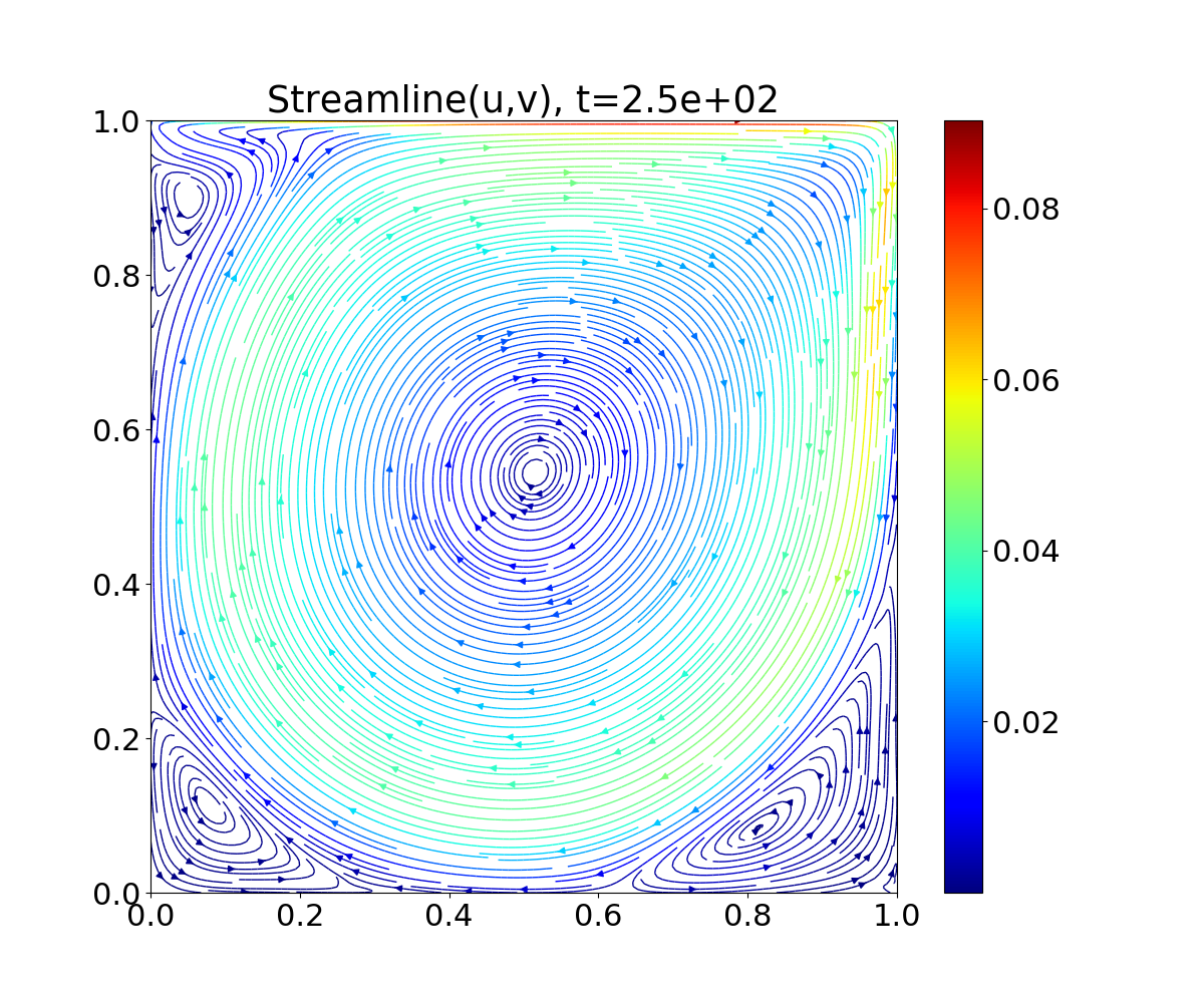
The provided Python script (Examples/Python/plotStreamlines_2DBinary.py) can be used to generate streamline plots from the binary file. Alternatively, HyPar::op_file_format can be set to tecplot2d, and Tecplot/VisIt or something similar can be used to plot the resulting files.
The following plot shows the final solution (velocity streamlines colored by the velocity magnitude):
The file function_counts.dat reports the computational expense (in terms of the number of function counts):
269
121110
121110
121110
4277
4277
2654
116833
The numbers are, respectively,
Expected screen output (for Reynolds number 3200):
srun: job 9980406 queued and waiting for resources
srun: job 9980406 has been allocated resources
HyPar - Parallel (MPI) version with 16 processes
Compiled with PETSc time integration.
Allocated simulation object(s).
Reading solver inputs from file "solver.inp".
No. of dimensions : 2
No. of variables : 4
Domain size : 128 128
Processes along each dimension : 4 4
Exact solution domain size : 128 128
No. of ghosts pts : 3
No. of iter. : 25000
Restart iteration : 0
Time integration scheme : PETSc
Spatial discretization scheme (hyperbolic) : upw5
Split hyperbolic flux term? : no
Interpolation type for hyperbolic term : components
Spatial discretization type (parabolic ) : nonconservative-2stage
Spatial discretization scheme (parabolic ) : 4
Time Step : 1.000000E-02
Check for conservation : no
Screen output iterations : 10
File output iterations : 100
Initial solution file type : binary
Initial solution read mode : serial
Solution file write mode : serial
Solution file format : binary
Overwrite solution file : yes
Physical model : navierstokes2d
Partitioning domain and allocating data arrays.
Reading array from binary file initial.inp (Serial mode).
Volume integral of the initial solution:
0: 1.0158100316200525E+00
1: -1.7347234759768071E-17
2: -8.6736173798840355E-19
3: 1.8148063242358203E+00
Reading boundary conditions from boundary.inp.
Boundary noslip-wall: Along dimension 0 and face +1
Boundary noslip-wall: Along dimension 0 and face -1
Boundary noslip-wall: Along dimension 1 and face +1
Boundary noslip-wall: Along dimension 1 and face -1
4 boundary condition(s) read.
Initializing solvers.
Initializing physics. Model = "navierstokes2d"
Reading physical model inputs from file "physics.inp".
Setting up PETSc time integration...
PETSc: total number of computational points is 16384.
PETSc: total number of computational DOFs is 65536.
Implicit-Explicit time-integration:-
Hyperbolic term: Implicit
Parabolic term: Implicit
Source term: Implicit
SolvePETSc(): Problem type is nonlinear.
** Starting PETSc time integration **
Writing solution file op.bin.
iter= 10 dt=4.525E-02 t=3.198E-01 CFL=6.262E+00 norm=3.0309E-02
iter= 20 dt=5.962E-02 t=8.389E-01 CFL=8.241E+00 norm=3.2289E-02
iter= 30 dt=7.221E-02 t=1.492E+00 CFL=1.015E+01 norm=3.3464E-02
iter= 40 dt=8.504E-02 t=2.273E+00 CFL=1.187E+01 norm=3.8478E-02
iter= 50 dt=9.766E-02 t=3.178E+00 CFL=1.360E+01 norm=4.0025E-02
iter= 60 dt=1.107E-01 t=4.210E+00 CFL=1.557E+01 norm=4.3005E-02
iter= 70 dt=1.232E-01 t=5.370E+00 CFL=1.740E+01 norm=3.7940E-02
iter= 80 dt=1.375E-01 t=6.668E+00 CFL=1.939E+01 norm=3.7970E-02
iter= 90 dt=1.507E-01 t=8.101E+00 CFL=2.119E+01 norm=3.9712E-02
iter= 100 dt=1.646E-01 t=9.677E+00 CFL=2.289E+01 norm=4.4672E-02
Writing solution file op.bin.
iter= 110 dt=1.798E-01 t=1.140E+01 CFL=2.523E+01 norm=2.3712E-02
iter= 120 dt=1.956E-01 t=1.328E+01 CFL=2.731E+01 norm=3.0056E-02
iter= 130 dt=2.123E-01 t=1.531E+01 CFL=2.975E+01 norm=3.0924E-02
iter= 140 dt=2.305E-01 t=1.751E+01 CFL=3.246E+01 norm=2.1651E-02
iter= 150 dt=2.505E-01 t=1.989E+01 CFL=3.484E+01 norm=2.8821E-02
iter= 160 dt=2.679E-01 t=2.247E+01 CFL=3.747E+01 norm=2.2700E-02
iter= 170 dt=2.914E-01 t=2.526E+01 CFL=4.049E+01 norm=3.7055E-02
iter= 180 dt=3.156E-01 t=2.827E+01 CFL=4.396E+01 norm=3.2539E-02
iter= 190 dt=3.463E-01 t=3.156E+01 CFL=4.831E+01 norm=2.8748E-02
iter= 200 dt=3.667E-01 t=3.512E+01 CFL=5.109E+01 norm=2.1596E-02
Writing solution file op.bin.
iter= 210 dt=3.916E-01 t=3.893E+01 CFL=5.466E+01 norm=2.0914E-02
iter= 220 dt=4.255E-01 t=4.299E+01 CFL=5.886E+01 norm=1.6388E-02
iter= 230 dt=4.671E-01 t=4.740E+01 CFL=6.490E+01 norm=1.6122E-02
iter= 240 dt=5.491E-01 t=5.238E+01 CFL=7.615E+01 norm=8.1433E-03
iter= 250 dt=8.980E-01 t=5.890E+01 CFL=1.246E+02 norm=1.3328E-03
iter= 260 dt=6.192E+01 t=1.187E+02 CFL=8.590E+03 norm=1.0463E-03
** Completed PETSc time integration **
Writing solution file op.bin.
Solver runtime (in seconds): 4.0300219099999998E+02
Total runtime (in seconds): 4.0305459200000001E+02
Deallocating arrays.
Finished.