See 1D Linear Advection - Discontinuous Waves to familiarize yourself with this case. This example uses a DMD object that has already been trained (see 1D Linear Advection - Discontinuous Waves (Time Windowed DMD)).

Location: hypar/Examples/1D/LinearAdvection/DiscontinuousWaves_libROM_DMD_Predict (This directory contains all the input files needed to run this case.)

Governing equations: 1D Linear Advection Equation (linearadr.h)

Reduced Order Modeling: This example predicts the solution from trained time-windowed DMD objects. The code does not solve the PDE by discretizing in space and integrating in time.

References:

Ghosh, D., Baeder, J. D., "Compact Reconstruction Schemes with Weighted ENO Limiting for Hyperbolic Conservation Laws", SIAM Journal on Scientific Computing, 34 (3), 2012, A1678–A1706

Domain: \(-1 \le x \le 1\), "periodic" (_PERIODIC_) boundary conditions

Initial solution:

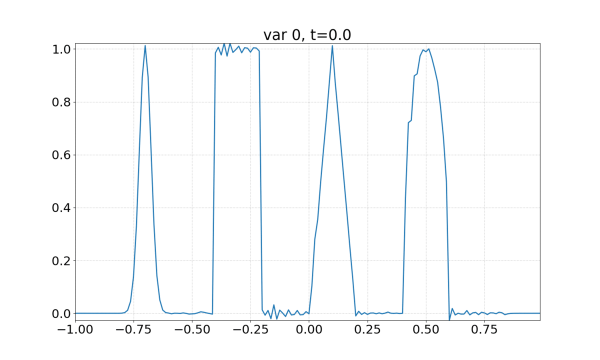
\begin{equation} u\left(x,0\right) = \left\{\begin{array}{lc} \exp\left(-\log\left(2\right)\frac{\left(x+7\right)^2}{0.0009}\right) & -0.8\le x \le -0.6 \\ 1 & -0.4\le x \le -0.2 \\ 1 - \left|10\left(x-0.1\right)\right| & 0\le x \le 0.2 \\ \sqrt{1-100\left(x-0.5\right)^2} & 0.4\le x \le 0.6 \\ 0 & {\rm otherwise} \end{array}\right. \end{equation}

Reduced Order Modeling:

Mode: predict (libROMInterface::m_mode, _ROM_MODE_PREDICT_)
Component Mode: monolithic (libROMInterface::m_comp_mode, _ROM_COMP_MODE_MONOLITHIC_)
Type: Dynamic Mode Decomposition (DMD) with time windowing (libROMInterface::m_rom_type)

Note:

In this mode, HyPar will run just like an usual PDE simulation, except that it will swap out the numerical spatial discretization and time integration with the ROM-based prediction. The input files and output files will be the same as a regular simulation with the following comments:

Numerical method inputs are ignored (eg. those that specify spatial discretization and time integration methods).
In solver.inp, the values for dt, n_iter, and file_op_iter is used only to compute the simulation times at which to compute and write the solution. The time step size, dt, need not respect any CFL criterion.
HyPar::ConservationCheck is set to "no" since it is not possible to compute conservation loss for a general domain (because boundary fluxes are not being computed).

Input files required:

librom.inp

begin
  mode          predict
  dmd_dirname   DMD
end

DMD Object(s) :
The trained DMD object(s) must be located in the directory specified in librom.inp as dmd_dirname (DMDROMObject::m_dirname). For this example, they were generated using 1D Linear Advection - Discontinuous Waves (Time Windowed DMD).

solver.inp

begin
  ndims             1
  nvars             1
  size              160
  iproc             4
  n_iter            20
  dt                0.1
  file_op_iter      1
  ip_file_type      ascii
  op_file_format    binary
  op_overwrite      no
  model             linear-advection-diffusion-reaction
end

boundary.inp

2
periodic      0     1     0     0
periodic      0    -1     0     0

physics.inp

begin
  advection 1.0
end

To generate initial.inp, compile and run the following code in the run directory. Note: if the final time is an integer multiple of the time period, the file initial.inp can also be used as the exact solution exact.inp (i.e. create a sym link called exact.inp pointing to initial.inp, or just copy initial.inp to exact.inp).

#include <stdio.h>
#include <stdlib.h>
#include <math.h>
#include <string.h>
double absolute(double x)
{
  return (x<0? -x : x);
}
int main(){
  
    int NI,ndims;
  char ip_file_type[50];
  strcpy(ip_file_type,"ascii");
  FILE *in;
  printf("Reading file \"solver.inp\"...\n");
  in = fopen("solver.inp","r");
  if (!in) printf("Error: Input file \"solver.inp\" not found. Default values will be used.\n");
  else {
    char word[500];
    fscanf(in,"%s",word);
    if (!strcmp(word, "begin")){
      while (strcmp(word, "end")){
        fscanf(in,"%s",word);
        if (!strcmp(word, "ndims"))             fscanf(in,"%d",&ndims);
        else if (!strcmp(word, "size"))         fscanf(in,"%d",&NI);
        else if (!strcmp(word, "ip_file_type")) fscanf(in,"%s",ip_file_type);
      }
    } else printf("Error: Illegal format in solver.inp. Crash and burn!\n");
  }
  fclose(in);
  if (ndims != 1) {
    printf("ndims is not 1 in solver.inp. this code is to generate 1D initial conditions\n");
    return(0);
  }
    printf("Grid:\t\t\t%d\n",NI);
    int i;
    double dx = 2.0 / ((double)NI);
    double *x, *u;
    x = (double*) calloc (NI, sizeof(double));
    u = (double*) calloc (NI, sizeof(double));
    for (i = 0; i < NI; i++){
        x[i] = -1.0 + i*dx;
    if      (x[i] < -0.8)  u[i] = 0.0;
    else if (x[i] < -0.6)  u[i] = exp(-log(2.0)*(x[i]+0.7)*(x[i]+0.7)/0.0009);
    else if (x[i] < -0.4)  u[i] = 0.0;
    else if (x[i] < -0.2)  u[i] = 1.0;
    else if (x[i] <  0  )  u[i] = 0.0;
    else if (x[i] <  0.2)  u[i] = 1.0 - absolute(10.0*(x[i]-0.1));
    else if (x[i] <  0.4)  u[i] = 0.0;
    else if (x[i] <  0.6)  u[i] = sqrt(1.0-100*(x[i]-0.5)*(x[i]-0.5));
    else                   u[i] = 0.0;
    }
  FILE *out;
  if (!strcmp(ip_file_type,"ascii")) {
    printf("Writing ASCII initial solution file initial.inp\n");
    out = fopen("initial.inp","w");
    for (i = 0; i < NI; i++)  fprintf(out,"%lf ",x[i]);
    fprintf(out,"\n");
      for (i = 0; i < NI; i++)  fprintf(out,"%lf ",u[i]);                       
    fprintf(out,"\n");
    fclose(out);
  } else if ((!strcmp(ip_file_type,"binary")) || (!strcmp(ip_file_type,"bin"))) {
    printf("Writing binary initial solution file initial.inp\n");
    out = fopen("initial.inp","wb");
    fwrite(x,sizeof(double),NI,out);
    fwrite(u,sizeof(double),NI,out);
    fclose(out);
  }
    free(x);
    free(u);
    return(0);
}

Output:

After running the code, there should be the following output files:

21 output files op_00000.bin, op_00001.bin, ... op_00020.bin; these are the solutions as predicted by the ROM .

The first of each of these file sets is the solution at \(t=0\) and the final one is the solution at \(t=3\). Since HyPar::op_overwrite is set to no in solver.inp, a separate file is written for solutions at each output time. All the files are binary (HyPar::op_file_format is set to binary in solver.inp).

The provided Python script (Examples/Python/plotSolution_1DBinary.py) can be used to generate plots from these binary files. Alternatively, HyPar::op_file_format can be set to text, and GNUPlot or something similar can be used to plot the resulting text files.

The animation shows the evolution of the solution.

Expected screen output:

HyPar - Parallel (MPI) version with 4 processes
Compiled with PETSc time integration.
Allocated simulation object(s).
Reading solver inputs from file "solver.inp".
  No. of dimensions                          : 1
  No. of variables                           : 1
  Domain size                                : 160 
  Processes along each dimension             : 4 
  Exact solution domain size                 : 160 
  No. of ghosts pts                          : 1
  No. of iter.                               : 20
  Restart iteration                          : 0
  Time integration scheme                    : euler 
  Spatial discretization scheme (hyperbolic) : 1
  Split hyperbolic flux term?                : no
  Interpolation type for hyperbolic term     : characteristic
  Spatial discretization type   (parabolic ) : nonconservative-1stage
  Spatial discretization scheme (parabolic ) : 2
  Time Step                                  : 1.000000E-01
  Check for conservation                     : no
  Screen output iterations                   : 1
  File output iterations                     : 1
  Initial solution file type                 : ascii
  Initial solution read mode                 : serial
  Solution file write mode                   : serial
  Solution file format                       : binary
  Overwrite solution file                    : no
  Physical model                             : linear-advection-diffusion-reaction
Partitioning domain and allocating data arrays.
Reading array from ASCII file initial.inp (Serial mode).
Volume integral of the initial solution:
 0:  5.1835172500000004E-01
Reading boundary conditions from boundary.inp.
  Boundary                       periodic:  Along dimension  0 and face +1
  Boundary                       periodic:  Along dimension  0 and face -1
2 boundary condition(s) read.
Initializing solvers.
Initializing physics. Model = "linear-advection-diffusion-reaction"
Reading physical model inputs from file "physics.inp".
Setting up libROM interface.
libROM inputs and parameters:
  reduced model dimensionality:  17867264
  sampling frequency:  0
  mode: predict
  type: DMD
  save to file: true
libROM DMD inputs:
  number of samples per window:   2147483647
  directory name for DMD onjects: DMD
libROMInterface::loadROM() - loading ROM objects.
  Loading DMD object (DMD/dmdobj_0000), time window=[0.00e+00,2.50e-01].
  Loading DMD object (DMD/dmdobj_0001), time window=[2.50e-01,5.00e-01].
  Loading DMD object (DMD/dmdobj_0002), time window=[5.00e-01,7.50e-01].
  Loading DMD object (DMD/dmdobj_0003), time window=[7.50e-01,1.00e+00].
  Loading DMD object (DMD/dmdobj_0004), time window=[1.00e+00,1.25e+00].
  Loading DMD object (DMD/dmdobj_0005), time window=[1.25e+00,1.50e+00].
  Loading DMD object (DMD/dmdobj_0006), time window=[1.50e+00,1.75e+00].
  Loading DMD object (DMD/dmdobj_0007), time window=[1.75e+00,-1.00e+00].
libROM: Predicted solution at time 0.0000e+00 using ROM, wallclock time: 0.000465.
Writing solution file op_00000.bin.
libROM: Predicted solution at time 1.0000e-01 using ROM, wallclock time: 0.052197.
Writing solution file op_00001.bin.
libROM: Predicted solution at time 2.0000e-01 using ROM, wallclock time: 0.069136.
Writing solution file op_00002.bin.
libROM: Predicted solution at time 3.0000e-01 using ROM, wallclock time: 0.120402.
Writing solution file op_00003.bin.
libROM: Predicted solution at time 4.0000e-01 using ROM, wallclock time: 0.032553.
Writing solution file op_00004.bin.
libROM: Predicted solution at time 5.0000e-01 using ROM, wallclock time: 0.086271.
Writing solution file op_00005.bin.
libROM: Predicted solution at time 6.0000e-01 using ROM, wallclock time: 0.078811.
Writing solution file op_00006.bin.
libROM: Predicted solution at time 7.0000e-01 using ROM, wallclock time: 0.097244.
Writing solution file op_00007.bin.
libROM: Predicted solution at time 8.0000e-01 using ROM, wallclock time: 0.121830.
Writing solution file op_00008.bin.
libROM: Predicted solution at time 9.0000e-01 using ROM, wallclock time: 0.053557.
Writing solution file op_00009.bin.
libROM: Predicted solution at time 1.0000e+00 using ROM, wallclock time: 0.078664.
Writing solution file op_00010.bin.
libROM: Predicted solution at time 1.1000e+00 using ROM, wallclock time: 0.058107.
Writing solution file op_00011.bin.
libROM: Predicted solution at time 1.2000e+00 using ROM, wallclock time: 0.084064.
Writing solution file op_00012.bin.
libROM: Predicted solution at time 1.3000e+00 using ROM, wallclock time: 0.111854.
Writing solution file op_00013.bin.
libROM: Predicted solution at time 1.4000e+00 using ROM, wallclock time: 0.059786.
Writing solution file op_00014.bin.
libROM: Predicted solution at time 1.5000e+00 using ROM, wallclock time: 0.101292.
Writing solution file op_00015.bin.
libROM: Predicted solution at time 1.6000e+00 using ROM, wallclock time: 0.093572.
Writing solution file op_00016.bin.
libROM: Predicted solution at time 1.7000e+00 using ROM, wallclock time: 0.095854.
Writing solution file op_00017.bin.
libROM: Predicted solution at time 1.8000e+00 using ROM, wallclock time: 0.141542.
Writing solution file op_00018.bin.
libROM: Predicted solution at time 1.9000e+00 using ROM, wallclock time: 0.081636.
Writing solution file op_00019.bin.
libROM: Predicted solution at time 2.0000e+00 using ROM, wallclock time: 0.089887.
Writing solution file op_00020.bin.
libROM: total prediction/query wallclock time: 1.708724 (seconds).
Solver runtime (in seconds): 2.7899449999999999E+00
Total  runtime (in seconds): 2.8098500000000000E+00
Deallocating arrays.
Finished.