See 2D Navier-Stokes Equations - Lid-Driven Square Cavity to familiarize yourself with this case. This example uses a DMD object that has already been trained (see 2D Navier-Stokes Equations - Lid-Driven Square Cavity (Time-Windowed DMD)).

Location: hypar/Examples/2D/NavierStokes2D/LidDrivenCavity_libROM_DMD_Predict (This directory contains all the input files needed to run this case.)

Governing equations: 2D Navier-Stokes Equations (navierstokes2d.h)

Reduced Order Modeling: This example predicts the solution from a trained DMD object. The code does not solve the PDE by discretizing in space and integrating in time.

Reference:

Erturk, E., Corke, T.C., and Gokcol, C., Numerical Solutions of 2-D Steady Incompressible Driven Cavity Flow at High Reynolds Numbers, International Journal for Numerical Methods in Fluids, 48, 2005, http://dx.doi.org/10.1002/fld.953.
Ghia, U., Ghia, K.N., Shin, C.T., High-Re Solutions for Incompressible Flow using the Navier-Stokes Equations and a Multigrid Method, Journal of Computational Physics, 48, 1982, http://dx.doi.org/10.1016/0021-9991(82)90058-4.

Note that this is an incompressible problem being solved here using the compressible Navier-Stokes equations in terms of non-dimensional flow variables. The density and pressure are taken such that the speed of sound is 1.0, and the flow velocities specified in the initial and boundary conditions correspond to a characteristic Mach number of 0.1 (thus, they are 0.1 times the values in the above reference).

Domain: \(0 \le x, y \le 1\)

Boundary conditions:

No-slip wall BC on \(x=0,1, 0 \le y \le 1\) (_NOSLIP_WALL_ with 0 wall velocity).
No-slip wall BC on \(y=0, 0 \le x \le 1\) (_NOSLIP_WALL_ with 0 wall velocity).
Moving no-slip wall BC on \(y=1, 0 \le x \le 1\) (_NOSLIP_WALL_ with specified wall velocity of 0.1 in the x-direction).

Initial solution: \(\rho=1, p=1/\gamma\). The velocities are specified according to the references above, but scaled by a factor of 0.1 to ensure that the characteristic Mach number is 0.1.

Other parameters:

\(\gamma = 1.4\) (NavierStokes2D::gamma)
\(Re = \frac {\rho u L } {\mu} = 100, 1000, 3200\) (Reynolds number) (NavierStokes2D::Re), where \(L=1\) is the cavity length and width.
\(Pr = 0.72\) (Prandtl number) (NavierStokes2D::Pr)
\(M_\infty = 0.1\) (characteristic Mach number) (NavierStokes2D::Minf)

Note: Pressure is taken as \(1/\gamma\) in the above so that the freestream speed of sound is 1.

Reduced Order Modeling:

Mode: predict (libROMInterface::m_mode, _ROM_MODE_PREDICT_)
Component Mode: monolithic (libROMInterface::m_comp_mode, _ROM_COMP_MODE_MONOLITHIC_)
Type: Dynamic Mode Decomposition (DMD) with time windowing (libROMInterface::m_rom_type)

Note:

In this mode, HyPar will run just like an usual PDE simulation, except that it will swap out the numerical spatial discretization and time integration with the ROM-based prediction. The input files and output files will be the same as a regular simulation with the following comments:

Numerical method inputs are ignored (eg. those that specify spatial discretization and time integration methods).
In solver.inp, the values for dt, n_iter, and file_op_iter is used only to compute the simulation times at which to compute and write the solution. The time step size, dt, need not respect any CFL criterion.
HyPar::ConservationCheck is set to "no" since it is not possible to compute conservation loss for a general domain (because boundary fluxes are not being computed).

Input files required:

librom.inp

begin
  mode            predict
  dmd_dirname     DMD
end

DMD Object(s) :
The trained DMD object(s) must be located in the directory specified in librom.inp as dmd_dirname (DMDROMObject::m_dirname). For this example, they were generated using 2D Navier-Stokes Equations - Lid-Driven Square Cavity (Time-Windowed DMD).

solver.inp

begin
  ndims               2
  nvars               4
  size                128 128
  iproc               4 4
  ghost               3
  par_space_type      nonconservative-2stage
  n_iter              1
  dt                  250.0
  screen_op_iter      1
  file_op_iter        1
  input_mode          serial
  ip_file_type        binary
  output_mode         serial
  op_file_format      binary
  op_overwrite        yes
  model               navierstokes2d
end

boundary.inp

4
noslip-wall   0     1     0     0      0   1.0
0.0 0.0
noslip-wall   0    -1     0     0      0   1.0
0.0 0.0
noslip-wall   1     1     0   1.0      0      0
0.0 0.0
noslip-wall   1    -1     0   1.0      0      0
0.1 0.0

physics.inp (Note: this file specifies \(Re = 3200\), change Re here for other Reynolds numbers.)

begin
  gamma     1.4
  upwinding roe
  Pr        0.72
  Minf      0.1
  Re        3200
end

To generate initial.inp (initial solution), compile and run the following code in the run directory

#include <stdio.h>
#include <stdlib.h>
#include <math.h>
#include <string.h>
int main()
{
  double gamma  = 1.4;
  
    int   NI,NJ,ndims;
  char  ip_file_type[50]; strcpy(ip_file_type,"ascii");
  FILE *in;
  printf("Reading file \"solver.inp\"...\n");
  in = fopen("solver.inp","r");
  if (!in) {
    printf("Error: Input file \"solver.inp\" not found. Default values will be used.\n");
    return(0);
  } else {
    char word[500];
    fscanf(in,"%s",word);
    if (!strcmp(word, "begin")) {
      while (strcmp(word, "end")) {
        fscanf(in,"%s",word);
        if (!strcmp(word, "ndims")) fscanf(in,"%d",&ndims);
        else if (!strcmp(word, "size")) {
          fscanf(in,"%d",&NI);
          fscanf(in,"%d",&NJ);
        } else if (!strcmp(word, "ip_file_type")) fscanf(in,"%s",ip_file_type);
      }
    } else printf("Error: Illegal format in solver.inp. Crash and burn!\n");
  }
  fclose(in);
  if (ndims != 2) {
    printf("ndims is not 2 in solver.inp. this code is to generate 2D initial conditions\n");
    return(0);
  }
    printf("Grid:\t\t\t%d X %d\n",NI,NJ);
    int i,j;
    double dx = 1.0 / ((double)NI-1);
    double dy = 1.0 / ((double)NJ-1);
  double Minf = 0.1;
    double *x, *y, *u0, *u1, *u2, *u3;
    x   = (double*) calloc (NI   , sizeof(double));
    y   = (double*) calloc (NJ   , sizeof(double));
    u0  = (double*) calloc (NI*NJ, sizeof(double));
    u1  = (double*) calloc (NI*NJ, sizeof(double));
    u2  = (double*) calloc (NI*NJ, sizeof(double));
    u3  = (double*) calloc (NI*NJ, sizeof(double));
    for (i = 0; i < NI; i++){
    for (j = 0; j < NJ; j++){
        x[i] = i*dx;
        y[j] = j*dy;
      int p = NJ*i + j;
      double rho, u, v, P;
      rho = 1.0;
      P   = 1.0/gamma;
      u   =   Minf * (y[j]-0.5);
      v   = - Minf * (x[i]-0.5);
      u0[p] = rho;
      u1[p] = rho*u;
      u2[p] = rho*v;
      u3[p] = P/(gamma-1.0) + 0.5*rho*(u*u+v*v);
      }
    }
  FILE *out;
  if (!strcmp(ip_file_type,"ascii")) {
    printf("Writing ASCII initial solution file initial.inp\n");
    out = fopen("initial.inp","w");
    for (i = 0; i < NI; i++)  fprintf(out,"%lf ",x[i]);
    fprintf(out,"\n");
    for (j = 0; j < NJ; j++)  fprintf(out,"%lf ",y[j]);
    fprintf(out,"\n");
    for (j = 0; j < NJ; j++)    {
        for (i = 0; i < NI; i++)    {
        int p = NJ*i + j;
        fprintf(out,"%lf ",u0[p]);
      }
    }
    fprintf(out,"\n");
    for (j = 0; j < NJ; j++)    {
        for (i = 0; i < NI; i++)    {
        int p = NJ*i + j;
        fprintf(out,"%lf ",u1[p]);
      }
    }
    fprintf(out,"\n");
    for (j = 0; j < NJ; j++)    {
        for (i = 0; i < NI; i++)    {
        int p = NJ*i + j;
        fprintf(out,"%lf ",u2[p]);
      }
    }
    fprintf(out,"\n");
    for (j = 0; j < NJ; j++)    {
        for (i = 0; i < NI; i++)    {
        int p = NJ*i + j;
        fprintf(out,"%lf ",u3[p]);
      }
    }
    fprintf(out,"\n");
      fclose(out);
  } else if ((!strcmp(ip_file_type,"binary")) || (!strcmp(ip_file_type,"bin"))) {
    printf("Writing binary initial solution file initial.inp\n");
    out = fopen("initial.inp","wb");
    fwrite(x,sizeof(double),NI,out);
    fwrite(y,sizeof(double),NJ,out);
    double *U = (double*) calloc (4*NI*NJ,sizeof(double));
    for (i=0; i < NI; i++) {
      for (j = 0; j < NJ; j++) {
        int p = NJ*i + j;
        int q = NI*j + i;
        U[4*q+0] = u0[p];
        U[4*q+1] = u1[p];
        U[4*q+2] = u2[p];
        U[4*q+3] = u3[p];
      }
    }
    fwrite(U,sizeof(double),4*NI*NJ,out);
    free(U);
    fclose(out);
  }
    free(x);
    free(y);
    free(u0);
    free(u1);
    free(u2);
    free(u3);
    return(0);
}

Output:

Note that iproc is set to

4 4

in solver.inp (i.e., 4 processors along x, and 4 processor along y). Thus, this example should be run with 16 MPI ranks (or change iproc).

After running the code, there should be the following output files:

1 output file op.bin; this is the solutions as predicted by the ROM .

It is a binary file. (HyPar::op_file_format is set to binary in solver.inp).

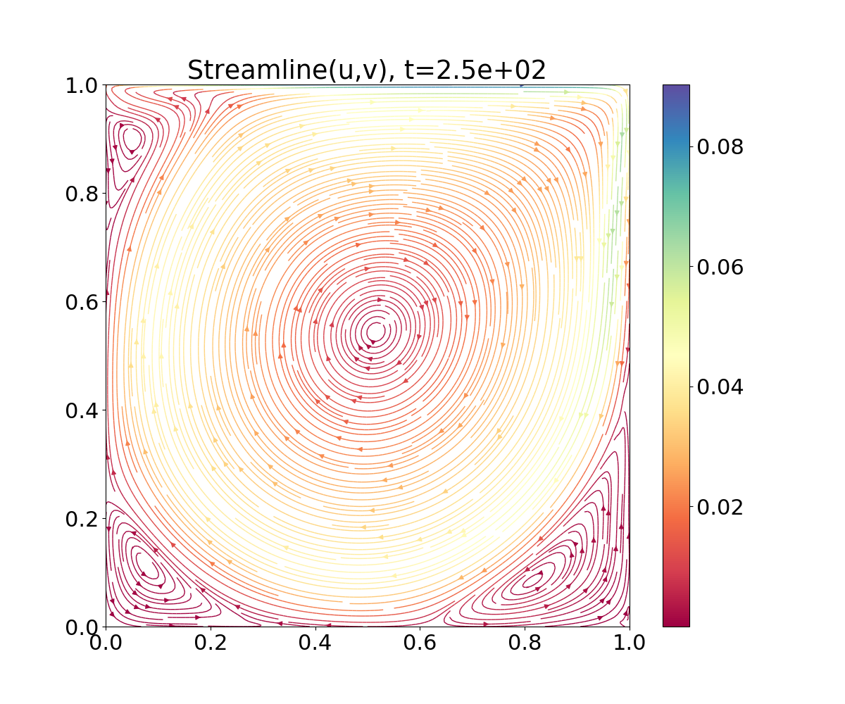
The provided Python script (Examples/Python/plotStreamlines_2DBinary.py) can be used to generate streamline plots from the binary file. Alternatively, HyPar::op_file_format can be set to tecplot2d, and Tecplot/VisIt or something similar can be used to plot the resulting files.

The following plot shows the final solution (velocity streamlines colored by the velocity magnitude):

Expected screen output:

HyPar - Parallel (MPI) version with 16 processes
Compiled with PETSc time integration.
Allocated simulation object(s).
Reading solver inputs from file "solver.inp".
  No. of dimensions                          : 2
  No. of variables                           : 4
  Domain size                                : 128 128 
  Processes along each dimension             : 4 4 
  Exact solution domain size                 : 128 128 
  No. of ghosts pts                          : 3
  No. of iter.                               : 1
  Restart iteration                          : 0
  Time integration scheme                    : euler 
  Spatial discretization scheme (hyperbolic) : 1
  Split hyperbolic flux term?                : no
  Interpolation type for hyperbolic term     : characteristic
  Spatial discretization type   (parabolic ) : nonconservative-2stage
  Spatial discretization scheme (parabolic ) : 2
  Time Step                                  : 2.500000E+02
  Check for conservation                     : no
  Screen output iterations                   : 1
  File output iterations                     : 1
  Initial solution file type                 : binary
  Initial solution read mode                 : serial
  Solution file write mode                   : serial
  Solution file format                       : binary
  Overwrite solution file                    : yes
  Physical model                             : navierstokes2d
Partitioning domain and allocating data arrays.
Reading array from binary file initial.inp (Serial mode).
Volume integral of the initial solution:
 0:  1.0158100316200525E+00
 1:  -1.7347234759768071E-17
 2:  -8.6736173798840355E-19
 3:  1.8148063242358203E+00
Reading boundary conditions from boundary.inp.
  Boundary                    noslip-wall:  Along dimension  0 and face +1
  Boundary                    noslip-wall:  Along dimension  0 and face -1
  Boundary                    noslip-wall:  Along dimension  1 and face +1
  Boundary                    noslip-wall:  Along dimension  1 and face -1
4 boundary condition(s) read.
Initializing solvers.
Initializing physics. Model = "navierstokes2d"
Reading physical model inputs from file "physics.inp".
Setting up libROM interface.
libROM inputs and parameters:
  reduced model dimensionality:  0
  sampling frequency:  0
  mode: predict
  type: DMD
  save to file: true
libROM DMD inputs:
  number of samples per window:   2147483647
  directory name for DMD onjects: DMD
libROMInterface::loadROM() - loading ROM objects.
  Loading DMD object (DMD/dmdobj_0000), time window=[0.00e+00,5.00e+01].
  Loading DMD object (DMD/dmdobj_0001), time window=[5.00e+01,1.00e+02].
  Loading DMD object (DMD/dmdobj_0002), time window=[1.00e+02,1.50e+02].
  Loading DMD object (DMD/dmdobj_0003), time window=[1.50e+02,2.00e+02].
  Loading DMD object (DMD/dmdobj_0004), time window=[2.00e+02,-1.00e+00].
libROM: Predicted solution at time 0.0000e+00 using ROM, wallclock time: 0.053045.
Writing solution file op.bin.
libROM: Predicted solution at time 2.5000e+02 using ROM, wallclock time: 0.146811.
Writing solution file op.bin.
libROM: total prediction/query wallclock time: 0.199856 (seconds).
Solver runtime (in seconds): 8.3036480000000008E+00
Total  runtime (in seconds): 8.6806149999999995E+00
Deallocating arrays.
Finished.