See 2D Euler Equations (with gravitational force) - Inertia-Gravity Waves to familiarize yourself with this case.
Location: hypar/Examples/2D/NavierStokes2D/InertiaGravityWave_PETSc_IMEX_libROM_DMD_Train (This directory contains all the input files needed to run this case.)
Governing equations: 2D Euler Equations (navierstokes2d.h - By default, NavierStokes2D::Re is set to -1 which makes the code skip the parabolic terms, i.e., the 2D Euler equations are solved.)
Reduced Order Modeling: This example trains a DMD object and then predicts the solution using the DMD at the same times that the actual HyPar solution is written at.
Reference:
- W. C. Skamarock and J. B. Klemp, "Efficiency and accuracy of
the Klemp-Wilhelmson timesplitting technique", Monthly Weather Review, 122 (1994), pp. 2623–2630.
- Giraldo, F.X., Restelli, M., "A study of spectral element and discontinuous Galerkin methods for the Navier–Stokes equations in nonhydrostatic mesoscale atmospheric modeling: Equation sets and test cases", J. Comput. Phys., 227, 2008, 3849–3877, (Section 3.1).
The problem is solved here using implicit-explicit (IMEX) time integration, where the hyperbolic flux is partitioned into its entropy and acoustic components with the former integrated explicitly and the latter integrated implicitly. See the following reference:
- Ghosh, D., Constantinescu, E. M., "Semi-Implicit Time Integration of
Atmospheric Flows with Characteristic-Based Flux Partitioning", SIAM Journal on Scientific Computing, 38 (3), 2016, A1848-A1875, http://dx.doi.org/10.1137/15M1044369.
Domain: \(0 \le x \le 300,000\,m, 0 \le y \le 10,000\,m\), "periodic" (_PERIODIC_) boundary conditions along \(x\), "slip-wall" (_SLIP_WALL_) boundary conditions along \(y\).
Initial solution: See references above.
Other parameters (all dimensional quantities are in SI units):
Numerical method:
Reduced Order Modeling:
Input files required:
librom.inp
begin
rdim 32
sampling_frequency 1
mode train
dmd_num_win_samples 50
end
.petscrc
# See PETSc documentation for more details (https://petsc.org/release/overview/).
# Note that if the following are specified in this file, the corresponding inputs in solver.inp are *ignored*.
# + "-ts_dt" (time step size): ignores "dt" in solver.inp
# + "-ts_max_steps" (maximum number of time iterations): ignores "n_iter" in solver.inp
# + "-ts_max_time" (final simulation time): ignores "n_iter" X "dt" in solver.inp
# Use PETSc time-integration
-use-petscts
# Time integration scheme type - ARK
-ts_type arkimex
-ts_arkimex_type 4
# Specify the terms to treat explicitly and implicitly
# In this example, the hyperbolic flux is partitioned
# into its entropy and acoustic components: f = [f-df] + [df]
# [f-df] - entropy component
# [df] - acoustic component
-hyperbolic_f_explicit # treat [f-df] explicitly
-hyperbolic_df_implicit # treat [df] implicitly
-source_implicit # treat source term implicitly
# thus, time step size is limited by the [f-df] term, i.e.,
# the flow velocity.
# no time-step adaptivity
-ts_adapt_type none
# For linear problens, tell nonlinear solver (SNES) to only use the linear solver (KSP)
-snes_type ksponly
# Linear solver (KSP) type
-ksp_type gmres
# Set relative tolerance
-ksp_rtol 1e-6
# Set absolute tolerance
-ksp_atol 1e-6
# use a preconditioner for solving the system
-with_pc
# preconditioner type - SOR
-pc_type sor
-pc_sor_omega 1.0
-pc_sor_its 2
# apply right preconditioner
-ksp_pc_side RIGHT
solver.inp
begin
ndims 2
nvars 4
size 1200 50
iproc 24 1
ghost 3
n_iter 300
restart_iter 0
hyp_space_scheme cupw5
hyp_flux_split yes
hyp_interp_type components
dt 10.0
screen_op_iter 10
file_op_iter 20
input_mode serial
ip_file_type binary
output_mode serial
op_file_format binary
op_overwrite no
model navierstokes2d
end
boundary.inp
4
periodic 0 1 0 0 0.0 10000.0
periodic 0 -1 0 0 0.0 10000.0
slip-wall 1 1 0.0 300000.0 0.0 0.0
0.0 0.0
slip-wall 1 -1 0.0 300000.0 0.0 0.0
0.0 0.0
physics.inp
begin
gamma 1.4
upwinding rusanov
gravity 0.0 9.8
rho_ref 1.1612055171196529
p_ref 100000.0
HB 3 0.01
R 287.058
end
To generate initial.inp (initial solution), compile and run the following code in the run directory.
#include <stdio.h>
#include <stdlib.h>
#include <math.h>
#include <string.h>
{
return(exp(a*log(x)));
}
{
double gamma = 1.4;
double R = 287.058;
double rho_ref = 1.1612055171196529;
double p_ref = 100000.0;
double grav_x = 0.0;
double grav_y = 9.8;
int HB = 0;
double BV = 0.0;
int NI,NK,ndims;
char ip_file_type[50];
strcpy(ip_file_type,"ascii");
FILE *in;
printf("Reading file \"solver.inp\"...\n");
in = fopen("solver.inp","r");
if (!in) {
printf ("Error: Input file \"solver.inp\" not found.\n");
return(1);
} else {
char word[500];
fscanf(in,"%s",word);
if (!strcmp(word, "begin")){
while (strcmp(word, "end")){
fscanf(in,"%s",word);
if (!strcmp(word, "ndims")) fscanf(in,"%d",&ndims);
else if (!strcmp(word, "size")) {
fscanf(in,"%d",&NI);
fscanf(in,"%d",&NK);
} else if (!strcmp(word, "ip_file_type")) fscanf(in,"%s",ip_file_type);
}
} else printf("Error: Illegal format in solver.inp. Crash and burn!\n");
}
fclose(in);
printf("Reading file \"physics.inp\"...\n");
in = fopen("physics.inp","r");
if (!in) {
printf("Error: Input file \"physics.inp\" not found.\n");
return(0);
} else {
char word[500];
fscanf(in,"%s",word);
if (!strcmp(word, "begin")) {
while (strcmp(word, "end")) {
fscanf(in,"%s",word);
if (!strcmp(word, "rho_ref")) fscanf(in,"%lf",&rho_ref);
else if (!strcmp(word, "p_ref" )) fscanf(in,"%lf",&p_ref );
else if (!strcmp(word, "gamma" )) fscanf(in,"%lf",&gamma );
else if (!strcmp(word, "R" )) fscanf(in,"%lf",&R );
else if (!strcmp(word, "HB" )) {
fscanf(in,"%d" ,&HB );
if (HB == 3) fscanf(in, "%lf", &BV);
} else if (!strcmp(word, "gravity")) {
fscanf(in,"%lf",&grav_x );
fscanf(in,"%lf",&grav_y );
}
}
} else printf("Error: Illegal format in physics.inp. Crash and burn!\n");
}
fclose(in);
if (ndims != 2) {
printf("ndims is not 2 in solver.inp. this code is to generate 2D initial conditions\n");
return(0);
}
if (HB != 3) {
printf("Error: Specify \"HB\" as 3 in physics.inp.\n");
}
if (grav_x != 0.0) {
printf("Error: Gravity force along x must be zero for HB = 3.\n");
return(0);
}
printf("Grid:\t\t\t%d X %d\n",NI,NK);
printf("Reference density and pressure: %lf, %lf.\n",rho_ref,p_ref);
double xmin, xmax, zmin, zmax;
xmin = 0.0;
xmax = 300000;
zmin = 0.0;
zmax = 10000.0 ;
double Lx = xmax - xmin;
double Lz = zmax - zmin;
int i,k;
double dx = Lx / ((double)NI-1);
double dz = Lz / ((double)NK-1);
double *x, *z, *U;
FILE *out;
x = (double*) calloc (NI , sizeof(double));
z = (double*) calloc (NK , sizeof(double));
U = (double*) calloc (4*NI*NK, sizeof(double));
double inv_gamma_m1 = 1.0 / (gamma-1.0);
double Cp = gamma * R * inv_gamma_m1;
double Cv = R * inv_gamma_m1;
double T_ref = p_ref / (R*rho_ref);
double pi = 4.0*atan(1.0);
double tc = 0.01;
double hc = 10000;
double ac = 5000;
double xc = 100000;
double uc = 20.0;
for (i = 0; i < NI; i++){
for (k = 0; k < NK; k++){
x[i] = xmin + i*dx;
z[k] = zmin + k*dz;
int p = i + NI*k;
double dtheta = tc * sin(pi*z[k]/hc) / (1.0 + ((x[i]-xc)/ac)*((x[i]-xc)/ac));
double theta = T_ref*exp(BV*BV*z[k]/grav_y) + dtheta;
double Pexner = 1.0 + ((grav_y*grav_y)/(Cp*T_ref*BV*BV))*(exp(-BV*BV*z[k]/grav_y)-1.0);
double rho = (p_ref/(R*theta)) *
raiseto(Pexner,inv_gamma_m1);
double E = Cv * theta * Pexner + 0.5 * (uc * uc);
U[4*p+0] = rho;
U[4*p+1] = rho*uc;
U[4*p+2] = 0.0;
U[4*p+3] = rho*E;
}
}
if (!strcmp(ip_file_type,"ascii")) {
printf("ASCII not supported. Use binary format\n");
} else if ((!strcmp(ip_file_type,"binary")) || (!strcmp(ip_file_type,"bin"))) {
printf("Writing binary initial solution file initial.inp\n");
out = fopen("initial.inp","wb");
fwrite(x,sizeof(double),NI,out);
fwrite(z,sizeof(double),NK,out);
fwrite(U,sizeof(double),4*NI*NK,out);
fclose(out);
}
free(x);
free(z);
free(U);
return(0);
}
Output:
Note that iproc is set to
24 1
in solver.inp (i.e., 24 processors along x, and 1 processor along y). Thus, this example should be run with 24 MPI ranks (or change iproc).
After running the code, there should be the following output files:
- 16 output file op_00000.bin, ..., op_00015.bin; this is the HyPar solutions.
- 16 output file op_rom_00000.bin, ..., op_rom_00015.bin; this is the predicted solutions from the DMD object(s).
All the files are binary (HyPar::op_file_format is set to binary in solver.inp).
HyPar::op_file_format is set to binary in solver.inp, and thus, all the files are written out in the binary format, see WriteBinary(). The binary file contains the conserved variables \(\left(\rho, \rho u, \rho v, e\right)\). The following code converts these variables to the primitive variables of interest to atmospheric flows \(\left(\rho, u, v, p, \theta\right)\). It also writes out the hydrostatically balanced quantities \(\left(\rho_0,\pi_0, \theta_0\right)\) for this case that can be used to compute and plot the temperature and density perturbations. These variables are then written to either a tecplot2d or text file. (compile and run it in the run directory):
#include <stdio.h>
#include <stdlib.h>
#include <string.h>
#include <math.h>
typedef struct _parameters_{
double g, R, gamma, P_ref, rho_ref, Nbv;
int HB;
} Parameters;
void IncrementFilename(char *f)
{
if (f[7] == '9') {
f[7] = '0';
if (f[6] == '9') {
f[6] = '0';
if (f[5] == '9') {
f[5] = '0';
if (f[4] == '9') {
f[4] = '0';
if (f[3] == '9') {
f[3] = '0';
fprintf(stderr,"Warning: file increment hit max limit. Resetting to zero.\n");
} else {
f[3]++;
}
} else {
f[4]++;
}
} else {
f[5]++;
}
} else {
f[6]++;
}
} else {
f[7]++;
}
}
{
return(exp(a*log(x)));
}
void WriteTecplot2D(
int nvars,
int imax,
int jmax,
double *x,
double *u,
char *f)
{
printf("\tWriting tecplot solution file %s.\n",f);
FILE *out;
out = fopen(f,"w");
if (!out) {
fprintf(stderr,"Error: could not open %s for writing.\n",f);
return;
}
double *X = x;
double *Y = x+imax;
fprintf(out,"VARIABLES=\"I\",\"J\",\"X\",\"Y\",");
fprintf(out,"\"RHO\",\"U\",\"V\",\"P\",");
fprintf(out,"\"THETA\",\"RHO0\",\"P0\",");
fprintf(out,"\"PI0\",\"THETA0\",\n");
fprintf(out,"ZONE I=%d,J=%d,F=POINT\n",imax,jmax);
int i,j;
for (j=0; j<jmax; j++) {
for (i=0; i<imax; i++) {
int v, p = i + imax*j;
fprintf(out,"%4d %4d ",i,j);
fprintf(out,"%1.16E %1.16E ",X[i],Y[j]);
for (v=0; v<nvars; v++) fprintf(out,"%1.16E ",u[nvars*p+v]);
fprintf(out,"\n");
}
}
fclose(out);
return;
}
void WriteText2D(int nvars,int imax, int jmax,double *x,double *u,char *f)
{
printf("\tWriting text solution file %s.\n",f);
FILE *out;
out = fopen(f,"w");
if (!out) {
fprintf(stderr,"Error: could not open %s for writing.\n",f);
return;
}
double *X = x;
double *Y = x+imax;
int i,j;
for (j=0; j<jmax; j++) {
for (i=0; i<imax; i++) {
int v, p = i + imax*j;
fprintf(out,"%4d %4d ",i,j);
fprintf(out,"%1.16E %1.16E ",X[i],Y[j]);
for (v=0; v<nvars; v++) fprintf(out,"%1.16E ",u[nvars*p+v]);
fprintf(out,"\n");
}
}
fclose(out);
return;
}
int PostProcess(char *fname, char *oname, void *p, int flag)
{
Parameters *params = (Parameters*) p;
FILE *in; in = fopen(fname,"rb");
if (!in) return(-1);
printf("Reading file %s.\n",fname);
int ndims, nvars;
double *U,*x;
fread(&ndims,sizeof(int),1,in);
fread(&nvars,sizeof(int),1,in);
if (ndims != 2) {
printf("Error: ndims in %s not equal to 2!\n",fname);
return(1);
}
if (nvars != 4) {
printf("Error: nvars in %s not equal to 4!\n",fname);
return(1);
}
int dims[ndims];
fread(dims,sizeof(int),ndims,in);
printf("Dimensions: %d x %d\n",dims[0],dims[1]);
printf("Nvars : %d\n",nvars);
x = (double*) calloc (dims[0]+dims[1] ,sizeof(double));
U = (double*) calloc (dims[0]*dims[1]*nvars ,sizeof(double));
fread(x,sizeof(double),dims[0]+dims[1] ,in);
fread(U,sizeof(double),dims[0]*dims[1]*nvars,in);
fclose(in);
int imax = dims[0];
int jmax = dims[1];
int evars = 5;
double *Q = (double*) calloc ((nvars+evars)*imax*jmax,sizeof(double));
int i, j;
double *X = x;
double *Y = x+imax;
double g = params->g;
double R = params->R;
double gamma = params->gamma;
double P_ref = params->P_ref;
double rho_ref = params->rho_ref;
double T_ref = P_ref / (R*rho_ref);
double inv_gamma_m1 = 1.0 / (gamma-1.0);
double Cp = gamma * inv_gamma_m1 * R;
double BV = params->Nbv;
for (i=0; i<imax; i++) {
for (j=0; j<jmax; j++) {
int p = i + imax*j;
double rho0, theta0, Pexner, P0;
Pexner = 1.0 + ((g*g)/(Cp*T_ref*BV*BV))*(exp(-BV*BV*Y[j]/g)-1.0);
theta0 = T_ref * exp(BV*BV*Y[j]/g);
P0 = P_ref *
raiseto(Pexner, gamma*inv_gamma_m1);
rho0 = rho_ref *
raiseto(Pexner, inv_gamma_m1 ) * exp(-BV*BV*Y[j]/g);
double rho, uvel, vvel, E, P, theta;
rho = U[nvars*p+0];
uvel = U[nvars*p+1] / rho;
vvel = U[nvars*p+2] / rho;
E = U[nvars*p+3];
P = (gamma-1.0) * (E - 0.5*rho*(uvel*uvel+vvel*vvel));
theta = (E-0.5*rho*(uvel*uvel+vvel*vvel))/(Pexner*rho) * ((gamma-1.0)/R);
Q[(nvars+evars)*p+0] = rho;
Q[(nvars+evars)*p+1] = uvel;
Q[(nvars+evars)*p+2] = vvel;
Q[(nvars+evars)*p+3] = P;
Q[(nvars+evars)*p+4] = theta;
Q[(nvars+evars)*p+5] = rho0;
Q[(nvars+evars)*p+6] = P0;
Q[(nvars+evars)*p+7] = Pexner;
Q[(nvars+evars)*p+8] = theta0;
}
}
else WriteText2D (nvars+evars,imax,jmax,x,Q,oname);
free(U);
free(Q);
free(x);
}
{
FILE *out1, *out2, *in, *inputs;
char filename[50], op_file_format[50], tecfile[50], overwrite[50];
int flag;
printf("Write tecplot file (1) or plain text file (0): ");
scanf("%d",&flag);
if ((flag != 1) && (flag != 0)) {
printf("Error: Invalid input. Should be 1 or 0.\n");
return(0);
}
printf("Reading solver.inp.\n");
inputs = fopen("solver.inp","r");
if (!inputs) {
fprintf(stderr,"Error: File \"solver.inp\" not found.\n");
return(1);
} else {
char word[100];
fscanf(inputs,"%s",word);
if (!strcmp(word, "begin")){
while (strcmp(word, "end")){
fscanf(inputs,"%s",word);
if (!strcmp(word, "op_file_format" )) fscanf(inputs,"%s" ,op_file_format);
else if (!strcmp(word, "op_overwrite" )) fscanf(inputs,"%s" ,overwrite );
}
}
fclose(inputs);
}
if (strcmp(op_file_format,"binary") && strcmp(op_file_format,"bin")) {
printf("Error: solution output needs to be in binary files.\n");
return(0);
}
Parameters params;
params.g = 9.8;
params.R = 287.058;
params.gamma = 1.4;
params.P_ref = 100000.0;
params.rho_ref = 100000.0 / (params.R * 300.0);
params.HB = 0;
params.Nbv = 0.0;
printf("Reading physics.inp.\n");
inputs = fopen("physics.inp","r");
if (!inputs) {
fprintf(stderr,"Error: File \"physics.inp\" not found.\n");
return(1);
} else {
char word[100];
fscanf(inputs,"%s",word);
if (!strcmp(word, "begin")){
while (strcmp(word, "end")){
fscanf(inputs,"%s",word);
if (!strcmp(word, "gamma")) fscanf(inputs,"%lf",¶ms.gamma);
else if (!strcmp(word, "gravity")) {
double crap; fscanf(inputs,"%lf",&crap);
fscanf(inputs,"%lf",¶ms.g);
} else if (!strcmp(word,"p_ref")) fscanf(inputs,"%lf",¶ms.P_ref);
else if (!strcmp(word,"rho_ref")) fscanf(inputs,"%lf",¶ms.rho_ref);
else if (!strcmp(word,"HB")) {
fscanf(inputs,"%d",¶ms.HB);
if (params.HB == 3) fscanf(inputs,"%lf",¶ms.Nbv);
}
}
}
fclose(inputs);
}
if (params.HB != 3) {
printf("Error: \"HB\" must be specified as 3 in physics.inp.\n");
return(0);
}
if (!strcmp(overwrite,"no")) {
strcpy(filename,"op_00000.bin");
while(1) {
strcpy(tecfile,filename);
tecfile[9] = 'd';
tecfile[10] = 'a';
tecfile[11] = 't';
int err = PostProcess(filename, tecfile, ¶ms, flag);
if (err == -1) {
printf("No more files found. Exiting.\n");
break;
}
IncrementFilename(filename);
}
} else if (!strcmp(overwrite,"yes")) {
strcpy(filename,"op.bin");
strcpy(tecfile,filename);
tecfile[3] = 'd';
tecfile[4] = 'a';
tecfile[5] = 't';
int err = PostProcess(filename, tecfile, ¶ms, flag);
if (err == -1) {
printf("Error: op.bin not found.\n");
return(0);
}
}
return(0);
}
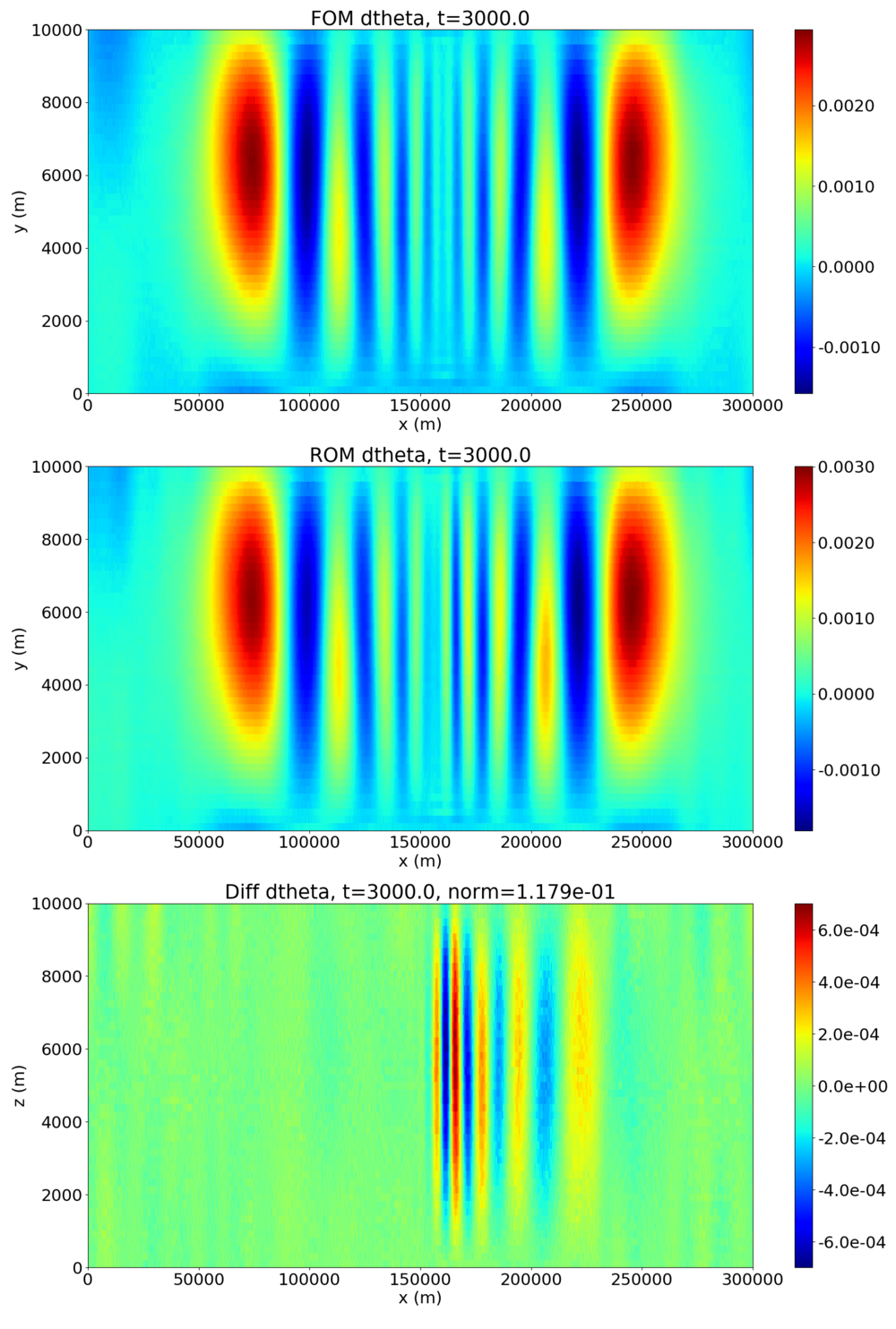
Alternatively, the provided Python script (plotSolution.py) can be used to generate plots from the binary files of the atmospheric flow variables and compare the HyPar and DMD solutions. It will plot the potential temperature perturbation but can be modified easily to plot other quantities.
The following plot shows the potential temperature perturbation contours at the final time t=3000 (FOM is the HyPar solution, ROM is the DMD prediction, and diff is the difference between the two):
Wall clock times:
- PDE solution: 521 seconds
- DMD training time: 15.1 seconds
- DMD prediction/query time: 8.7 seconds
The L1, L2, and Linf norms of the diff between the HyPar and ROM solution at the final time are calculated and reported on screen (see below) as well as pde_rom_diff.dat:
1200 50 24 1 1.0000000000000000E+01 1.6823397339748363E-07 2.0644508136507202E-07 6.2271161570040760E-07 5.4798857799999996E+02 5.4807861200000002E+02
The numbers are: number of grid points in each dimension (HyPar::dim_global), number of processors in each dimension (MPIVariables::iproc), time step size (HyPar::dt), L1, L2, and L-infinity norms of the diff (HyPar::rom_diff_norms), solver wall time (seconds) (i.e., not accounting for initialization, and cleaning up), and total wall time.
Expected screen output:
srun: job 10160167 queued and waiting for resources
srun: job 10160167 has been allocated resources
HyPar - Parallel (MPI) version with 24 processes
Compiled with PETSc time integration.
Allocated simulation object(s).
Reading solver inputs from file "solver.inp".
No. of dimensions : 2
No. of variables : 4
Domain size : 1200 50
Processes along each dimension : 24 1
Exact solution domain size : 1200 50
No. of ghosts pts : 3
No. of iter. : 300
Restart iteration : 0
Time integration scheme : PETSc
Spatial discretization scheme (hyperbolic) : cupw5
Split hyperbolic flux term? : yes
Interpolation type for hyperbolic term : components
Spatial discretization type (parabolic ) : nonconservative-1stage
Spatial discretization scheme (parabolic ) : 2
Time Step : 1.000000E+01
Check for conservation : no
Screen output iterations : 10
File output iterations : 20
Initial solution file type : binary
Initial solution read mode : serial
Solution file write mode : serial
Solution file format : binary
Overwrite solution file : no
Physical model : navierstokes2d
Partitioning domain and allocating data arrays.
Reading array from binary file initial.inp (Serial mode).
Volume integral of the initial solution:
0: 2.2722878895077395E+09
1: 4.5445757790154785E+10
2: 0.0000000000000000E+00
3: 4.4309563899845638E+14
Reading boundary conditions from boundary.inp.
Boundary periodic: Along dimension 0 and face +1
Boundary periodic: Along dimension 0 and face -1
Boundary slip-wall: Along dimension 1 and face +1
Boundary slip-wall: Along dimension 1 and face -1
4 boundary condition(s) read.
Initializing solvers.
tridiagLUInit: File "lusolver.inp" not found. Using default values.
Initializing physics. Model = "navierstokes2d"
Reading physical model inputs from file "physics.inp".
Setting up PETSc time integration...
Setting up libROM interface.
libROMInterface inputs and parameters:
reduced model dimensionality: 32
sampling frequency: 1
mode: train
component mode: monolithic
type: DMD
save to file: true
DMDROMObject details:
number of samples per window: 50
directory name for DMD onjects: DMD
write snapshot matrix to file: false
simulation domain: 0
PETSc: total number of computational points is 60000.
PETSc: total number of computational DOFs is 240000.
Implicit-Explicit time-integration:-
Hyperbolic (f-df) term: Explicit
Hyperbolic (df) term: Implicit
Parabolic term: Implicit
Source term: Implicit
SolvePETSc(): Problem type is linear.
** Starting PETSc time integration **
Writing solution file op_00000.bin.
DMDROMObject::takeSample() - creating new DMD object for sim. domain 0, var -1, t=0.000000 (total: 1).
iter= 10 dt=1.000E+01 t=1.000E+02 CFL=1.701E+01 norm=1.0002E-01 wctime: 1.7E+00 (s)
iter= 20 dt=1.000E+01 t=2.000E+02 CFL=1.701E+01 norm=1.6347E-01 wctime: 1.7E+00 (s)
Writing solution file op_00001.bin.
iter= 30 dt=1.000E+01 t=3.000E+02 CFL=1.701E+01 norm=1.4808E-01 wctime: 1.7E+00 (s)
iter= 40 dt=1.000E+01 t=4.000E+02 CFL=1.701E+01 norm=1.1472E-01 wctime: 1.7E+00 (s)
Writing solution file op_00002.bin.
iter= 50 dt=1.000E+01 t=5.000E+02 CFL=1.701E+01 norm=1.0850E-01 wctime: 1.7E+00 (s)
DMDROMObject::train() - training DMD object 0 for sim. domain 0, var -1 with 51 samples.
Using 32 basis vectors out of 50.
DMDROMObject::takeSample() - creating new DMD object for sim. domain 0, var -1, t=500.000000 (total: 2).
iter= 60 dt=1.000E+01 t=6.000E+02 CFL=1.701E+01 norm=1.4884E-01 wctime: 1.7E+00 (s)
Writing solution file op_00003.bin.
iter= 70 dt=1.000E+01 t=7.000E+02 CFL=1.701E+01 norm=1.4899E-01 wctime: 1.7E+00 (s)
iter= 80 dt=1.000E+01 t=8.000E+02 CFL=1.701E+01 norm=1.1894E-01 wctime: 1.7E+00 (s)
Writing solution file op_00004.bin.
iter= 90 dt=1.000E+01 t=9.000E+02 CFL=1.701E+01 norm=1.0875E-01 wctime: 1.7E+00 (s)
iter= 100 dt=1.000E+01 t=1.000E+03 CFL=1.701E+01 norm=1.4186E-01 wctime: 1.7E+00 (s)
Writing solution file op_00005.bin.
DMDROMObject::train() - training DMD object 1 for sim. domain 0, var -1 with 51 samples.
Using 32 basis vectors out of 50.
DMDROMObject::takeSample() - creating new DMD object for sim. domain 0, var -1, t=1000.000000 (total: 3).
iter= 110 dt=1.000E+01 t=1.100E+03 CFL=1.701E+01 norm=1.4984E-01 wctime: 1.7E+00 (s)
iter= 120 dt=1.000E+01 t=1.200E+03 CFL=1.701E+01 norm=1.3136E-01 wctime: 1.7E+00 (s)
Writing solution file op_00006.bin.
iter= 130 dt=1.000E+01 t=1.300E+03 CFL=1.701E+01 norm=1.1261E-01 wctime: 1.7E+00 (s)
iter= 140 dt=1.000E+01 t=1.400E+03 CFL=1.701E+01 norm=1.3477E-01 wctime: 1.7E+00 (s)
Writing solution file op_00007.bin.
iter= 150 dt=1.000E+01 t=1.500E+03 CFL=1.701E+01 norm=1.3695E-01 wctime: 1.7E+00 (s)
DMDROMObject::train() - training DMD object 2 for sim. domain 0, var -1 with 51 samples.
Using 32 basis vectors out of 50.
DMDROMObject::takeSample() - creating new DMD object for sim. domain 0, var -1, t=1500.000000 (total: 4).
iter= 160 dt=1.000E+01 t=1.600E+03 CFL=1.701E+01 norm=1.4525E-01 wctime: 1.7E+00 (s)
Writing solution file op_00008.bin.
iter= 170 dt=1.000E+01 t=1.700E+03 CFL=1.701E+01 norm=1.0836E-01 wctime: 1.7E+00 (s)
iter= 180 dt=1.000E+01 t=1.800E+03 CFL=1.701E+01 norm=1.1849E-01 wctime: 1.7E+00 (s)
Writing solution file op_00009.bin.
iter= 190 dt=1.000E+01 t=1.900E+03 CFL=1.701E+01 norm=1.5889E-01 wctime: 1.7E+00 (s)
iter= 200 dt=1.000E+01 t=2.000E+03 CFL=1.701E+01 norm=1.3183E-01 wctime: 1.7E+00 (s)
Writing solution file op_00010.bin.
DMDROMObject::train() - training DMD object 3 for sim. domain 0, var -1 with 51 samples.
Using 32 basis vectors out of 50.
DMDROMObject::takeSample() - creating new DMD object for sim. domain 0, var -1, t=2000.000000 (total: 5).
iter= 210 dt=1.000E+01 t=2.100E+03 CFL=1.701E+01 norm=1.1340E-01 wctime: 1.7E+00 (s)
iter= 220 dt=1.000E+01 t=2.200E+03 CFL=1.701E+01 norm=1.3901E-01 wctime: 1.7E+00 (s)
Writing solution file op_00011.bin.
iter= 230 dt=1.000E+01 t=2.300E+03 CFL=1.701E+01 norm=1.2231E-01 wctime: 1.7E+00 (s)
iter= 240 dt=1.000E+01 t=2.400E+03 CFL=1.701E+01 norm=1.3908E-01 wctime: 1.7E+00 (s)
Writing solution file op_00012.bin.
iter= 250 dt=1.000E+01 t=2.500E+03 CFL=1.701E+01 norm=1.2931E-01 wctime: 1.7E+00 (s)
DMDROMObject::train() - training DMD object 4 for sim. domain 0, var -1 with 51 samples.
Using 32 basis vectors out of 50.
DMDROMObject::takeSample() - creating new DMD object for sim. domain 0, var -1, t=2500.000000 (total: 6).
iter= 260 dt=1.000E+01 t=2.600E+03 CFL=1.701E+01 norm=1.3253E-01 wctime: 1.7E+00 (s)
Writing solution file op_00013.bin.
iter= 270 dt=1.000E+01 t=2.700E+03 CFL=1.701E+01 norm=1.1236E-01 wctime: 1.7E+00 (s)
iter= 280 dt=1.000E+01 t=2.800E+03 CFL=1.701E+01 norm=1.5150E-01 wctime: 1.7E+00 (s)
Writing solution file op_00014.bin.
iter= 290 dt=1.000E+01 t=2.900E+03 CFL=1.701E+01 norm=1.4059E-01 wctime: 1.7E+00 (s)
iter= 300 dt=1.000E+01 t=3.000E+03 CFL=1.701E+01 norm=1.0576E-01 wctime: 1.7E+00 (s)
Writing solution file op_00015.bin.
** Completed PETSc time integration (Final time: 3000.000000), total wctime: 521.165210 (seconds) **
DMDROMObject::train() - training DMD object 5 for sim. domain 0, var -1 with 50 samples.
Using 32 basis vectors out of 49.
libROM: total training wallclock time: 15.078729 (seconds).
libROM: Predicted solution at time 0.0000e+00 using ROM, wallclock time: 0.530589.
Writing solution file op_rom_00000.bin.
libROM: Predicted solution at time 2.0000e+02 using ROM, wallclock time: 0.598458.
Writing solution file op_rom_00001.bin.
libROM: Predicted solution at time 4.0000e+02 using ROM, wallclock time: 0.558467.
Writing solution file op_rom_00002.bin.
libROM: Predicted solution at time 6.0000e+02 using ROM, wallclock time: 0.495275.
Writing solution file op_rom_00003.bin.
libROM: Predicted solution at time 8.0000e+02 using ROM, wallclock time: 0.492773.
Writing solution file op_rom_00004.bin.
libROM: Predicted solution at time 1.0000e+03 using ROM, wallclock time: 0.495487.
Writing solution file op_rom_00005.bin.
libROM: Predicted solution at time 1.2000e+03 using ROM, wallclock time: 0.495699.
Writing solution file op_rom_00006.bin.
libROM: Predicted solution at time 1.4000e+03 using ROM, wallclock time: 0.497169.
Writing solution file op_rom_00007.bin.
libROM: Predicted solution at time 1.6000e+03 using ROM, wallclock time: 0.518542.
Writing solution file op_rom_00008.bin.
libROM: Predicted solution at time 1.8000e+03 using ROM, wallclock time: 0.518565.
Writing solution file op_rom_00009.bin.
libROM: Predicted solution at time 2.0000e+03 using ROM, wallclock time: 0.503544.
Writing solution file op_rom_00010.bin.
libROM: Predicted solution at time 2.2000e+03 using ROM, wallclock time: 0.500226.
Writing solution file op_rom_00011.bin.
libROM: Predicted solution at time 2.4000e+03 using ROM, wallclock time: 0.518636.
Writing solution file op_rom_00012.bin.
libROM: Predicted solution at time 2.6000e+03 using ROM, wallclock time: 0.498987.
Writing solution file op_rom_00013.bin.
libROM: Predicted solution at time 2.8000e+03 using ROM, wallclock time: 0.496688.
Writing solution file op_rom_00014.bin.
libROM: Predicted solution at time 3.0000e+03 using ROM, wallclock time: 0.494127.
Writing solution file op_rom_00015.bin.
libROM: Predicted solution at time 3.0000e+03 using ROM, wallclock time: 0.499386.
libROM: Calculating diff between PDE and ROM solutions.
Writing solution file op_rom_00016.bin.
libROM: total prediction/query wallclock time: 8.712618 (seconds).
libROMInterface::saveROM() - saving ROM objects.
Saving DMD object and summary (DMD/dmdobj_0000, DMD/dmd_summary_0000).
Saving DMD object and summary (DMD/dmdobj_0001, DMD/dmd_summary_0001).
Saving DMD object and summary (DMD/dmdobj_0002, DMD/dmd_summary_0002).
Saving DMD object and summary (DMD/dmdobj_0003, DMD/dmd_summary_0003).
Saving DMD object and summary (DMD/dmdobj_0004, DMD/dmd_summary_0004).
Saving DMD object and summary (DMD/dmdobj_0005, DMD/dmd_summary_0005).
Norms of the diff between ROM and PDE solutions for domain 0:
L1 Norm : 1.6823397339748363E-07
L2 Norm : 2.0644508136507202E-07
Linfinity Norm : 6.2271161570040760E-07
Solver runtime (in seconds): 5.4798857799999996E+02
Total runtime (in seconds): 5.4807861200000002E+02
Deallocating arrays.
Finished.