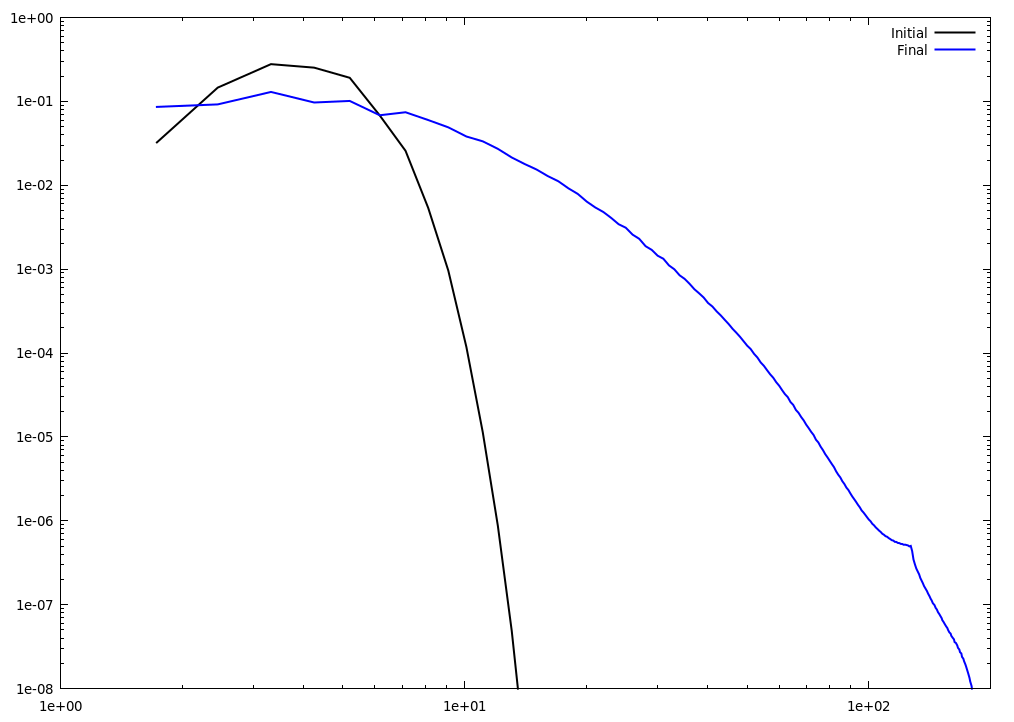
Initial solution: Isotropic turbulent flow - The initial solution is specified in the Fourier space (with an energy distribution similar to that of turbulent flow), and then transformed to the physical space through an inverse transform.
(see the FFTW website on ways to install it).
#include <stdio.h>
#include <stdlib.h>
#include <string.h>
#include <math.h>
#include <fftw3.h>
static const double PI = 4 * atan(1.0);
double raiseto(
double x,
double a) {
return exp(a*log(x));
}
double magnitude(double a, double b) {
return sqrt(a*a + b*b);
}
void velocityComponent( const int N,
const int dir,
const double kp,
const double u0,
double* const uvel )
{
long N3 = N*N*N;
long i,j,k;
double kk = sqrt(3 * (N/2)*(N/2));
int kkmax = (int) kk;
fftw_complex *uhat = (fftw_complex*) fftw_malloc(N3 * sizeof(fftw_complex));
fftw_complex *u = (fftw_complex*) fftw_malloc(N3 * sizeof(fftw_complex));
fftw_plan inv_trans_u;
inv_trans_u = fftw_plan_dft_3d(N, N, N, uhat, u, 1, FFTW_MEASURE);
for (i=0; i<N3; i++) uhat[i][0] = uhat[i][1] = 0.0;
for (i = 1; i < N/2; i++){
for (j = 0; j < N/2; j++){
for (k = 0; k < N/2; k++){
double kk = sqrt(i*i + j*j + k*k);
double th1 = 2*PI * ((double)rand())/((double)RAND_MAX);
double th2 = 2*PI * ((double)rand())/((double)RAND_MAX);
double phi1 = 2*PI * ((double)rand())/((double)RAND_MAX);
double E = 16.0 * sqrt(2.0/PI) * (u0*u0/kp) *
raiseto(kk/kp, 4.0)
* exp(-2.0*(kk/kp)*(kk/kp));
double alfa_real = sqrt(E/(4*PI*kk*kk))*cos(th1)*cos(phi1);
double alfa_imag = sqrt(E/(4*PI*kk*kk))*sin(th1)*cos(phi1);
double beta_real = sqrt(E/(4*PI*kk*kk))*cos(th2)*sin(phi1);
double beta_imag = sqrt(E/(4*PI*kk*kk))*sin(th2)*sin(phi1);
if (dir == 0) {
uhat[k+N*(j+N*i)][0] = (alfa_real*kk*j+beta_real*i*k)/(kk*sqrt(i*i+j*j));
uhat[k+N*(j+N*i)][1] = (alfa_imag*kk*j+beta_imag*i*k)/(kk*sqrt(i*i+j*j));
} else if (dir == 1) {
uhat[k+N*(j+N*i)][0] = (beta_real*j*k-alfa_real*kk*i)/(kk*sqrt(i*i+j*j));
uhat[k+N*(j+N*i)][1] = (beta_imag*j*k-alfa_imag*kk*i)/(kk*sqrt(i*i+j*j));
} else {
uhat[k+N*(j+N*i)][0] = -(beta_real*sqrt(i*i+j*j))/kk;
uhat[k+N*(j+N*i)][1] = -(beta_imag*sqrt(i*i+j*j))/kk;
}
}
}
}
for (i = 0; i < 1; i++){
for (k = 0; k < N/2; k++){
for (j = 1; j < N/2; j++){
double kk = sqrt(i*i + j*j + k*k);
double th1 = 2*PI * ((double)rand())/((double)RAND_MAX);
double th2 = 2*PI * ((double)rand())/((double)RAND_MAX);
double phi1 = 2*PI * ((double)rand())/((double)RAND_MAX);
double E = 16.0 * sqrt(2.0/PI) * (u0*u0/kp) *
raiseto(kk/kp, 4.0)
* exp(-2.0*(kk/kp)*(kk/kp));
double alfa_real = sqrt(E/(4*PI*kk*kk))*cos(th1)*cos(phi1);
double alfa_imag = sqrt(E/(4*PI*kk*kk))*sin(th1)*cos(phi1);
double beta_real = sqrt(E/(4*PI*kk*kk))*cos(th2)*sin(phi1);
double beta_imag = sqrt(E/(4*PI*kk*kk))*sin(th2)*sin(phi1);
if (dir == 0) {
uhat[k+N*(j+N*i)][0] = (alfa_real*kk*j+beta_real*i*k)/(kk*sqrt(i*i+j*j));
uhat[k+N*(j+N*i)][1] = (alfa_imag*kk*j+beta_imag*i*k)/(kk*sqrt(i*i+j*j));
} else if (dir == 1) {
uhat[k+N*(j+N*i)][0] = (beta_real*j*k-alfa_real*kk*i)/(kk*sqrt(i*i+j*j));
uhat[k+N*(j+N*i)][1] = (beta_imag*j*k-alfa_imag*kk*i)/(kk*sqrt(i*i+j*j));
} else {
uhat[k+N*(j+N*i)][0] = -(beta_real*sqrt(i*i+j*j))/kk;
uhat[k+N*(j+N*i)][1] = -(beta_imag*sqrt(i*i+j*j))/kk;
}
}
}
}
for (i = 0; i < 1; i++){
for (j = 0; j < 1; j++){
for (k = 0; k < N/2; k++){
uhat[k+N*(j+N*i)][0] = 0;
uhat[k+N*(j+N*i)][1] = 0;
}
}
}
for (i=N/2+1; i<N; i++) {
for (j=N/2+1; j<N; j++) {
for (k=N/2+1; k<N; k++) {
uhat[k+N*(j+N*i)][0] = uhat[(N-k)+N*((N-j)+N*(N-i))][0];
uhat[k+N*(j+N*i)][1] = -uhat[(N-k)+N*((N-j)+N*(N-i))][1];
}
}
}
for (i=N/2+1; i<N; i++) {
for (j=N/2+1; j<N; j++) {
for (k=0; k<1; k++) {
uhat[k+N*(j+N*i)][0] = uhat[k+N*((N-j)+N*(N-i))][0];
uhat[k+N*(j+N*i)][1] = -uhat[k+N*((N-j)+N*(N-i))][1];
}
}
}
for (i=N/2+1; i<N; i++) {
for (j=0; j<1; j++) {
for (k=N/2+1; k<N; k++) {
uhat[k+N*(j+N*i)][0] = uhat[(N-k)+N*(j+N*(N-i))][0];
uhat[k+N*(j+N*i)][1] = -uhat[(N-k)+N*(j+N*(N-i))][1];
}
}
}
for (i=0; i<1; i++) {
for (j=N/2+1; j<N; j++) {
for (k=N/2+1; k<N; k++) {
uhat[k+N*(j+N*i)][0] = uhat[(N-k)+N*((N-j)+N*i)][0];
uhat[k+N*(j+N*i)][1] = -uhat[(N-k)+N*((N-j)+N*i)][1];
}
}
}
for (i=0; i<1; i++) {
for (j=0; j<1; j++) {
for (k=N/2+1; k<N; k++) {
uhat[k+N*(j+N*i)][0] = uhat[(N-k)+N*(j+N*i)][0];
uhat[k+N*(j+N*i)][1] = -uhat[(N-k)+N*(j+N*i)][1];
}
}
}
for (i=0; i<1; i++) {
for (j=N/2+1; j<N; j++) {
for (k=0; k<1; k++) {
uhat[k+N*(j+N*i)][0] = uhat[k+N*((N-j)+N*i)][0];
uhat[k+N*(j+N*i)][1] = -uhat[k+N*((N-j)+N*i)][1];
}
}
}
for (i=N/2+1; i<N; i++) {
for (j=0; j<1; j++) {
for (k=0; k<1; k++) {
uhat[k+N*(j+N*i)][0] = uhat[k+N*(j+N*(N-i))][0];
uhat[k+N*(j+N*i)][1] = -uhat[k+N*(j+N*(N-i))][1];
}
}
}
fftw_execute(inv_trans_u);
fftw_free(uhat);
fftw_destroy_plan(inv_trans_u);
double imag_velocity = 0;
for (i = 0; i < N3; i++){
double uu = u[i][1];
imag_velocity += (uu*uu);
}
imag_velocity = sqrt(imag_velocity / ((double)N3));
printf("RMS of imaginary component of computed velocity: %1.6e\n",imag_velocity);
for (i = 0; i < N3; i++){
uvel[i] = u[i][0];
}
fftw_free(u);
return;
}
void setVelocityField(const int N,
double* const uvel,
double* const vvel,
double* const wvel )
{
double kp = 4.0;
double u0 = 0.3;
long N3 = N*N*N;
long i,j,k;
double dx = 2*PI / ((double)N);
velocityComponent( N, 0, kp, u0, uvel );
velocityComponent( N, 1, kp, u0, vvel );
velocityComponent( N, 2, kp, u0, wvel );
double rms_velocity = 0;
for (i = 0; i < N3; i++){
double uu, vv, ww;
uu = uvel[i];
vv = vvel[i];
ww = wvel[i];
rms_velocity += (uu*uu + vv*vv + ww*ww);
}
rms_velocity = sqrt(rms_velocity / (3*((double)N3)));
double factor = u0 / rms_velocity;
printf("Scaling factor = %1.16E\n",factor);
for (i = 0; i < N3; i++){
uvel[i] *= factor;
vvel[i] *= factor;
wvel[i] *= factor;
}
rms_velocity = 0;
for (i = 0; i < N3; i++){
double uu, vv, ww;
uu = uvel[i];
vv = vvel[i];
ww = wvel[i];
rms_velocity += (uu*uu + vv*vv + ww*ww);
}
rms_velocity = sqrt(rms_velocity / (3*((double)N3)));
printf("RMS velocity (component-wise): %1.16E\n",rms_velocity);
double DivergenceNorm = 0;
for (i=0; i<N; i++) {
for (j=0; j<N; j++) {
for (k=0; k<N; k++) {
double u1, u2, v1, v2, w1, w2;
u1 = (i==0 ? uvel[k+N*(j+N*(N-1))] : uvel[k+N*(j+N*(i-1))] );
u2 = (i==N-1 ? uvel[k+N*(j+N*(0 ))] : uvel[k+N*(j+N*(i+1))] );
v1 = (j==0 ? vvel[k+N*((N-1)+N*i)] : vvel[k+N*((j-1)+N*i)] );
v2 = (j==N-1 ? vvel[k+N*((0 )+N*i)] : vvel[k+N*((j+1)+N*i)] );
w1 = (k==0 ? wvel[(N-1)+N*(j+N*i)] : wvel[(k-1)+N*(j+N*i)] );
w2 = (k==N-1 ? wvel[(0 )+N*(j+N*i)] : wvel[(k+1)+N*(j+N*i)] );
double Divergence = ( (u2-u1) + (v2-v1) + (w2-w1) ) / (2.0*dx);
DivergenceNorm += (Divergence*Divergence);
}
}
}
DivergenceNorm = sqrt(DivergenceNorm / ((double)N3));
printf("Velocity divergence: %1.16E\n",DivergenceNorm);
double TaylorMicroscale[3];
double Numerator[3] = {0,0,0};
double Denominator[3] = {0,0,0};
for (i=0; i<N; i++) {
for (j=0; j<N; j++) {
for (k=0; k<N; k++) {
double u1, u2, uu, v1, v2, vv, w1, w2, ww;
u1 = (i==0 ? uvel[k+N*(j+N*(N-1))] : uvel[k+N*(j+N*(i-1))] );
u2 = (i==N-1 ? uvel[k+N*(j+N*(0 ))] : uvel[k+N*(j+N*(i+1))] );
v1 = (j==0 ? vvel[k+N*((N-1)+N*i)] : vvel[k+N*((j-1)+N*i)] );
v2 = (j==N-1 ? vvel[k+N*((0 )+N*i)] : vvel[k+N*((j+1)+N*i)] );
w1 = (k==0 ? wvel[(N-1)+N*(j+N*i)] : wvel[(k-1)+N*(j+N*i)] );
w2 = (k==N-1 ? wvel[(0 )+N*(j+N*i)] : wvel[(k+1)+N*(j+N*i)] );
uu = uvel[k+N*(j+N*i)];
vv = vvel[k+N*(j+N*i)];
ww = wvel[k+N*(j+N*i)];
double du, dv, dw;
du = (u2 - u1) / (2.0*dx);
dv = (v2 - v1) / (2.0*dx);
dw = (w2 - w1) / (2.0*dx);
Numerator[0] += (uu*uu);
Numerator[1] += (vv*vv);
Numerator[2] += (ww*ww);
Denominator[0] += (du*du);
Denominator[1] += (dv*dv);
Denominator[2] += (dw*dw);
}
}
}
Numerator[0] /= (N*N*N); Denominator[0] /= (N*N*N);
Numerator[1] /= (N*N*N); Denominator[1] /= (N*N*N);
Numerator[2] /= (N*N*N); Denominator[2] /= (N*N*N);
TaylorMicroscale[0] = sqrt(Numerator[0]/Denominator[0]);
TaylorMicroscale[1] = sqrt(Numerator[1]/Denominator[1]);
TaylorMicroscale[2] = sqrt(Numerator[2]/Denominator[2]);
printf("Taylor microscales: %1.16E, %1.16E, %1.16E\n",
TaylorMicroscale[0],TaylorMicroscale[1],TaylorMicroscale[2]);
return;
}
{
FILE *out, *in;
int NI,NJ,NK,ndims;
char ip_file_type[50];
strcpy(ip_file_type,"ascii");
printf("Reading file \"solver.inp\"...\n");
in = fopen("solver.inp","r");
if (!in) printf("Error: Input file \"solver.inp\" not found. Default values will be used.\n");
else {
char word[500];
fscanf(in,"%s",word);
if (!strcmp(word, "begin")){
while (strcmp(word, "end")){
fscanf(in,"%s",word);
if (!strcmp(word, "ndims")) fscanf(in,"%d",&ndims);
else if (!strcmp(word, "size")) {
fscanf(in,"%d",&NI);
fscanf(in,"%d",&NJ);
fscanf(in,"%d",&NK);
} else if (!strcmp(word, "ip_file_type")) fscanf(in,"%s",ip_file_type);
}
} else printf("Error: Illegal format in solver.inp. Crash and burn!\n");
}
fclose(in);
if (ndims != 3) {
printf("ndims is not 3 in solver.inp. this code is to generate 3D exact conditions\n");
return(0);
}
printf("Grid:\t\t\t%d x %d x %d\n",NI,NJ,NK);
if ((NI != NJ) || (NI != NK) || (NJ != NK)) {
printf("Error: NI,NJ,NK not equal. Bye!\n");
return(0);
}
int N = NI;
long N3 = N*N*N;
int i,j,k;
double dx = 2*PI / ((double)N);
double* u = (double*) calloc (N3, sizeof(double));
double* v = (double*) calloc (N3, sizeof(double));
double* w = (double*) calloc (N3, sizeof(double));
setVelocityField(N, u, v, w);
double *x,*y,*z,*U;
x = (double*) calloc (N, sizeof(double));
y = (double*) calloc (N, sizeof(double));
z = (double*) calloc (N, sizeof(double));
U = (double*) calloc (5*N3, sizeof(double));
for (i = 0; i < N; i++){
for (j = 0; j < N; j++){
for (k = 0; k < N; k++){
x[i] = i*dx;
y[j] = j*dx;
z[k] = k*dx;
double RHO, uvel, vvel, wvel, P;
RHO = 1.0;
uvel = u[k+N*(j+N*i)];
vvel = v[k+N*(j+N*i)];
wvel = w[k+N*(j+N*i)];
P = 1.0/1.4;
long p = i + N*j + N*N*k;
U[5*p+0] = RHO;
U[5*p+1] = RHO*uvel;
U[5*p+2] = RHO*vvel;
U[5*p+3] = RHO*wvel;
U[5*p+4] = P/0.4 + 0.5 * RHO * (uvel*uvel + vvel*vvel + wvel*wvel);
}
}
}
free(u);
free(v);
free(w);
FILE *op;
if (!strcmp(ip_file_type,"ascii")) {
printf("Writing ASCII initial solution file initial.inp\n");
op = fopen("initial.inp","w");
for (i = 0; i < N; i++) fprintf(op,"%1.16E ",x[i]);
fprintf(op,"\n");
for (j = 0; j < N; j++) fprintf(op,"%1.16E ",y[j]);
fprintf(op,"\n");
for (k = 0; k < N; k++) fprintf(op,"%1.16E ",z[k]);
fprintf(op,"\n");
for (i = 0; i < N; i++) {
for (j = 0; j < N; j++) {
for (k = 0; k < N; k++) {
int p = i + N*j + N*N*k;
fprintf(op,"%1.16E ",U[5*p+0]);
}
}
}
fprintf(op,"\n");
for (i = 0; i < N; i++) {
for (j = 0; j < N; j++) {
for (k = 0; k < N; k++) {
int p = i + N*j + N*N*k;
fprintf(op,"%1.16E ",U[5*p+1]);
}
}
}
fprintf(op,"\n");
for (i = 0; i < N; i++) {
for (j = 0; j < N; j++) {
for (k = 0; k < N; k++) {
int p = i + N*j + N*N*k;
fprintf(op,"%1.16E ",U[5*p+2]);
}
}
}
fprintf(op,"\n");
for (i = 0; i < N; i++) {
for (j = 0; j < N; j++) {
for (k = 0; k < N; k++) {
int p = i + N*j + N*N*k;
fprintf(op,"%1.16E ",U[5*p+3]);
}
}
}
fprintf(op,"\n");
for (i = 0; i < N; i++) {
for (j = 0; j < N; j++) {
for (k = 0; k < N; k++) {
int p = i + N*j + N*N*k;
fprintf(op,"%1.16E ",U[5*p+4]);
}
}
}
fprintf(op,"\n");
fclose(op);
} else if ((!strcmp(ip_file_type,"binary")) || (!strcmp(ip_file_type,"bin"))) {
printf("Writing binary initial solution file initial.inp\n");
op = fopen("initial.inp","wb");
fwrite(x,sizeof(double),N,op);
fwrite(y,sizeof(double),N,op);
fwrite(z,sizeof(double),N,op);
fwrite(U,sizeof(double),5*N3,op);
fclose(op);
}
free(x);
free(y);
free(z);
free(U);
return(0);
}
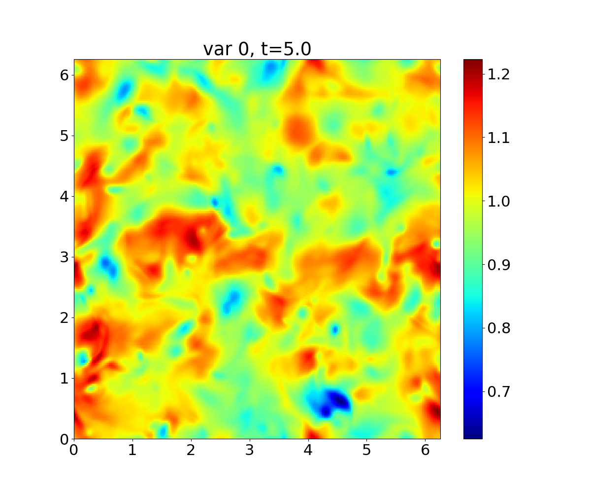
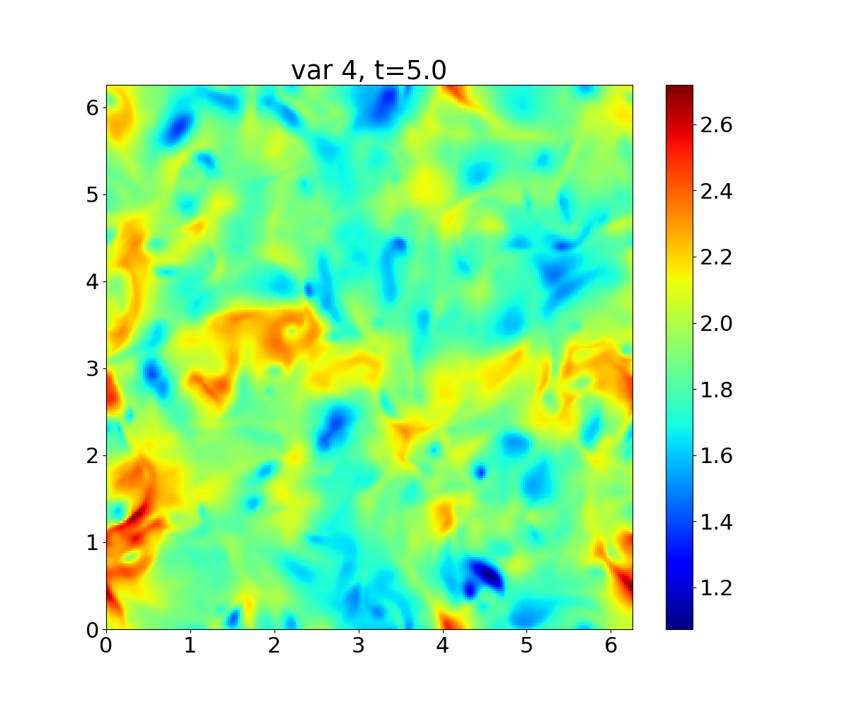
The following figures show the density and internal energy contours on the X-Y plane mid-slice at the final time:
HyPar - Parallel (MPI) version with 64 processes
Allocated simulation object(s).
Reading solver inputs from file "solver.inp".
No. of dimensions : 3
No. of variables : 5
Domain size : 256 256 256
Processes along each dimension : 4 4 4
Exact solution domain size : 256 256 256
No. of ghosts pts : 3
No. of iter. : 1000
Restart iteration : 0
Time integration scheme : rk (ssprk3)
Spatial discretization scheme (hyperbolic) : weno5
Split hyperbolic flux term? : no
Interpolation type for hyperbolic term : components
Spatial discretization type (parabolic ) : nonconservative-2stage
Spatial discretization scheme (parabolic ) : 4
Time Step : 5.000000E-03
Check for conservation : no
Screen output iterations : 50
File output iterations : 100
Initial solution file type : binary
Initial solution read mode : serial
Solution file write mode : serial
Solution file format : binary
Overwrite solution file : no
Use GPU : yes
GPU device no : 0
Physical model : navierstokes3d
Partitioning domain and allocating data arrays.
Reading array from binary file initial.inp (Serial mode).
Volume integral of the initial solution:
0: 2.4805021344162057E+02
1: 3.6748382115092681E-14
2: 5.6732396558345499E-14
3: 3.9412917374193057E-14
4: 4.7643358853329369E+02
Reading boundary conditions from boundary.inp.
Boundary periodic: Along dimension 0 and face +1
Boundary periodic: Along dimension 0 and face -1
Boundary periodic: Along dimension 1 and face +1
Boundary periodic: Along dimension 1 and face -1
Boundary periodic: Along dimension 2 and face +1
Boundary periodic: Along dimension 2 and face -1
6 boundary condition(s) read.
Initializing solvers.
Reading WENO parameters from weno.inp.
Initializing physics. Model = "navierstokes3d"
Reading physical model inputs from file "physics.inp".
Setting up time integration.
Solving in time (from 0 to 1000 iterations)
Writing solution file op_00000.bin.
iter= 50 t=2.500E-01 wctime: 8.3E-02 (s)
iter= 100 t=5.000E-01 wctime: 8.2E-02 (s)
Writing solution file op_00001.bin.
iter= 150 t=7.500E-01 wctime: 8.2E-02 (s)
iter= 200 t=1.000E+00 wctime: 8.3E-02 (s)
Writing solution file op_00002.bin.
iter= 250 t=1.250E+00 wctime: 8.3E-02 (s)
iter= 300 t=1.500E+00 wctime: 8.3E-02 (s)
Writing solution file op_00003.bin.
iter= 350 t=1.750E+00 wctime: 8.2E-02 (s)
iter= 400 t=2.000E+00 wctime: 8.2E-02 (s)
Writing solution file op_00004.bin.
iter= 450 t=2.250E+00 wctime: 8.2E-02 (s)
iter= 500 t=2.500E+00 wctime: 8.2E-02 (s)
Writing solution file op_00005.bin.
iter= 550 t=2.750E+00 wctime: 8.3E-02 (s)
iter= 600 t=3.000E+00 wctime: 8.2E-02 (s)
Writing solution file op_00006.bin.
iter= 650 t=3.250E+00 wctime: 8.2E-02 (s)
iter= 700 t=3.500E+00 wctime: 8.3E-02 (s)
Writing solution file op_00007.bin.
iter= 750 t=3.750E+00 wctime: 8.3E-02 (s)
iter= 800 t=4.000E+00 wctime: 8.3E-02 (s)
Writing solution file op_00008.bin.
iter= 850 t=4.250E+00 wctime: 8.2E-02 (s)
iter= 900 t=4.500E+00 wctime: 8.2E-02 (s)
Writing solution file op_00009.bin.
iter= 950 t=4.750E+00 wctime: 8.3E-02 (s)
iter= 1000 t=5.000E+00 wctime: 8.2E-02 (s)
Completed time integration (Final time: 5.000000), total wctime: 82.421372 (seconds).
Writing solution file op_00010.bin.
Solver runtime (in seconds): 9.5411868999999996E+01
Total runtime (in seconds): 1.0222746800000000E+02
Deallocating arrays.
Finished.