Characteristic-based 3rd-order MUSCL scheme with Koren's limiter. More...
#include <stdio.h>#include <stdlib.h>#include <basic.h>#include <arrayfunctions.h>#include <matmult_native.h>#include <mathfunctions.h>#include <interpolation.h>#include <mpivars.h>#include <hypar.h>Go to the source code of this file.
Macros | |
| #define | _MINIMUM_GHOSTS_ 3 |
Functions | |
| int | Interp1PrimThirdOrderMUSCLChar (double *fI, double *fC, double *u, double *x, int upw, int dir, void *s, void *m, int uflag) |
| 3rd order MUSCL scheme with Koren's limiter (characteristic-based) on a uniform grid More... | |
Detailed Description
Characteristic-based 3rd-order MUSCL scheme with Koren's limiter.
Definition in file Interp1PrimThirdOrderMUSCLChar.c.
Macro Definition Documentation
◆ _MINIMUM_GHOSTS_
| #define _MINIMUM_GHOSTS_ 3 |
Minimum number of ghost points required for this interpolation method.
Definition at line 25 of file Interp1PrimThirdOrderMUSCLChar.c.
Function Documentation
◆ Interp1PrimThirdOrderMUSCLChar()
| int Interp1PrimThirdOrderMUSCLChar | ( | double * | fI, |
| double * | fC, | ||
| double * | u, | ||
| double * | x, | ||
| int | upw, | ||
| int | dir, | ||
| void * | s, | ||
| void * | m, | ||
| int | uflag | ||
| ) |
3rd order MUSCL scheme with Koren's limiter (characteristic-based) on a uniform grid
Computes the interpolated values of the first primitive of a function \({\bf f}\left({\bf u}\right)\) at the interfaces from the cell-centered values of the function using the 3rd order MUSCL scheme with Koren's limiter on a uniform grid. The first primitive is defined as a function \({\bf h}\left({\bf u}\right)\) that satisfies:
\begin{equation} {\bf f}\left({\bf u}\left(x\right)\right) = \frac{1}{\Delta x} \int_{x-\Delta x/2}^{x+\Delta x/2} {\bf h}\left({\bf u}\left(\zeta\right)\right)d\zeta, \end{equation}
where \(x\) is the spatial coordinate along the dimension of the interpolation. This function computes numerical approximation \(\hat{\bf f}_{j+1/2} \approx {\bf h}_{j+1/2}\) as: using the 3rd order MUSCL scheme with Koren's limiter as follows:
\begin{equation} \hat{\alpha}^k_{j+1/2} = {\alpha}^k_{j-1} + \phi \left[\frac{1}{3}\left({\alpha}^k_j-{\alpha}^k_{j-1}\right) + \frac{1}{6}\left({\alpha}^k_{j-1}-{\alpha}^k_{j-2}\right)\right] \end{equation}
where
\begin{equation} \phi = \frac {3\left({\alpha}^k_j-{\alpha}^k_{j-1}\right)\left({\alpha}^k_{j-1}-{\alpha}^k_{j-2}\right) + \epsilon} {2\left[\left({\alpha}^k_j-{\alpha}^k_{j-1}\right)-\left({\alpha}^k_{j-1}-{\alpha}^k_{j-2}\right)\right]^2 + 3\left({\alpha}^k_j-{\alpha}^k_{j-1}\right)\left({\alpha}^k_{j-1}-{\alpha}^k_{j-2}\right) + \epsilon}, \end{equation}
\(\epsilon\) is a small constant (typically \(10^{-3}\)), and
\begin{equation} \alpha^k = {\bf l}_k \cdot {\bf f},\ k=1,\cdots,n \end{equation}
is the \(k\)-th characteristic quantity, and \({\bf l}_k\) is the \(k\)-th left eigenvector, \({\bf r}_k\) is the \(k\)-th right eigenvector, and \(n\) is HyPar::nvars. The final interpolated function is computed from the interpolated characteristic quantities as:
\begin{equation} \hat{\bf f}_{j+1/2} = \sum_{k=1}^n \alpha^k_{j+1/2} {\bf r}_k \end{equation}
Implementation Notes:
- This method assumes a uniform grid in the spatial dimension corresponding to the interpolation.
- The method described above corresponds to a left-biased interpolation. The corresponding right-biased interpolation can be obtained by reflecting the equations about interface j+1/2.
The left and right eigenvectors are computed at an averaged quantity at j+1/2. Thus, this function requires functions to compute the average state, and the left and right eigenvectors. These are provided by the physical model through
If these functions are not provided by the physical model, then a characteristic-based interpolation cannot be used.
- The function computes the interpolant for the entire grid in one call. It loops over all the grid lines along the interpolation direction and carries out the 1D interpolation along these grid lines.
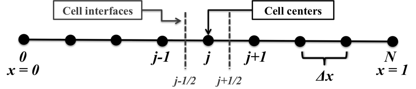
- Location of cell-centers and cell interfaces along the spatial dimension of the interpolation is shown in the following figure:
Function arguments:
| Argument | Type | Explanation ------— |
|---|---|---|
| fI | double* | Array to hold the computed interpolant at the grid interfaces. This array must have the same layout as the solution, but with no ghost points. Its size should be the same as u in all dimensions, except dir (the dimension along which to interpolate) along which it should be larger by 1 (number of interfaces is 1 more than the number of interior cell centers). |
| fC | double* | Array with the cell-centered values of the flux function \({\bf f}\left({\bf u}\right)\). This array must have the same layout and size as the solution, with ghost points. |
| u | double* | The solution array \({\bf u}\) (with ghost points). If the interpolation is characteristic based, this is needed to compute the eigendecomposition. For a multidimensional problem, the layout is as follows: u is a contiguous 1D array of size (nvars*dim[0]*dim[1]*...*dim[D-1]) corresponding to the multi-dimensional solution, with the following ordering - nvars, dim[0], dim[1], ..., dim[D-1], where nvars is the number of solution components (HyPar::nvars), dim is the local size (HyPar::dim_local), D is the number of spatial dimensions. |
| x | double* | The grid array (with ghost points). This is used only by non-uniform-grid interpolation methods. For multidimensional problems, the layout is as follows: x is a contiguous 1D array of size (dim[0]+dim[1]+...+dim[D-1]), with the spatial coordinates along dim[0] stored from 0,...,dim[0]-1, the spatial coordinates along dim[1] stored along dim[0],...,dim[0]+dim[1]-1, and so forth. |
| upw | int | Upwinding direction: if positive, a left-biased interpolant will be computed; if negative, a right-biased interpolant will be computed. If the interpolation method is central, then this has no effect. |
| dir | int | Spatial dimension along which to interpolate (eg: 0 for 1D; 0 or 1 for 2D; 0,1 or 2 for 3D) |
| s | void* | Solver object of type HyPar: the following variables are needed - HyPar::ghosts, HyPar::ndims, HyPar::nvars, HyPar::dim_local. |
| m | void* | MPI object of type MPIVariables: this is needed only by compact interpolation method that need to solve a global implicit system across MPI ranks. |
| uflag | int | A flag indicating if the function being interpolated \({\bf f}\) is the solution itself \({\bf u}\) (if 1, \({\bf f}\left({\bf u}\right) \equiv {\bf u}\)). |
Reference:
- van Leer, B., Towards the Ultimate Conservative Difference Scheme. 2: Monotonicity and Conservation Combined in a Second-Order Scheme, J. of Comput. Phys., 14 (4), 1974, pp.361-370, http://dx.doi.org/10.1016/0021-9991(74)90019-9
- Koren, B., A Robust Upwind Discretization Method for Advection, Diffusion and Source Terms, Centrum voor Wiskunde en Informatica, Amsterdam, 1993
- Parameters
-
fI Array of interpolated function values at the interfaces fC Array of cell-centered values of the function \({\bf f}\left({\bf u}\right)\) u Array of cell-centered values of the solution \({\bf u}\) x Grid coordinates upw Upwind direction (left or right biased) dir Spatial dimension along which to interpolation s Object of type HyPar containing solver-related variables m Object of type MPIVariables containing MPI-related variables uflag Flag to indicate if \(f(u) \equiv u\), i.e, if the solution is being reconstructed
Definition at line 91 of file Interp1PrimThirdOrderMUSCLChar.c.