|
HyPar
1.0
Finite-Difference Hyperbolic-Parabolic PDE Solver on Cartesian Grids
|
|
HyPar
1.0
Finite-Difference Hyperbolic-Parabolic PDE Solver on Cartesian Grids
|
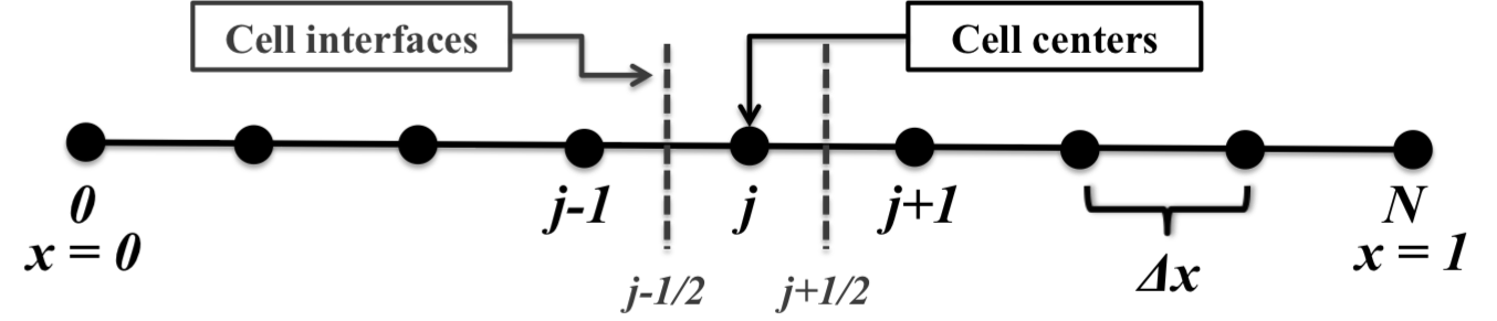
Definitions for the functions computing the interpolated value of the primitive at the cell interfaces from the cell-centered values. More...
#include "basic.h"Go to the source code of this file.
Data Structures | |
| struct | MUSCLParameters |
| Structure of variables/parameters needed by the MUSCL scheme. More... | |
| struct | WENOParameters |
| Structure of variables/parameters needed by the WENO-type scheme. More... | |
| struct | CompactScheme |
| Structure of variables/parameters needed by the compact schemes. More... | |
Macros | |
| #define | _FIRST_ORDER_UPWIND_ "1" |
| #define | _SECOND_ORDER_CENTRAL_ "2" |
| #define | _SECOND_ORDER_MUSCL_ "muscl2" |
| #define | _THIRD_ORDER_MUSCL_ "muscl3" |
| #define | _FOURTH_ORDER_CENTRAL_ "4" |
| #define | _FIFTH_ORDER_UPWIND_ "upw5" |
| #define | _FIFTH_ORDER_COMPACT_UPWIND_ "cupw5" |
| #define | _FIFTH_ORDER_WENO_ "weno5" |
| #define | _FIFTH_ORDER_CRWENO_ "crweno5" |
| #define | _FIFTH_ORDER_HCWENO_ "hcweno5" |
| #define | _CHARACTERISTIC_ "characteristic" |
| #define | _COMPONENTS_ "components" |
| #define | _WENO_OPTIMAL_WEIGHT_1_ 0.1 |
| #define | _WENO_OPTIMAL_WEIGHT_2_ 0.6 |
| #define | _WENO_OPTIMAL_WEIGHT_3_ 0.3 |
| #define | _CRWENO_OPTIMAL_WEIGHT_1_ 0.2 |
| #define | _CRWENO_OPTIMAL_WEIGHT_2_ 0.5 |
| #define | _CRWENO_OPTIMAL_WEIGHT_3_ 0.3 |
| #define | _WENOWeights_v_JS_(w1, w2, w3, c1, c2, c3, m3, m2, m1, p1, p2, eps, N) |
| #define | _WENOWeights_v_M_(w1, w2, w3, c1, c2, c3, m3, m2, m1, p1, p2, eps, N) |
| #define | _WENOWeights_v_M_Scalar_(w1, w2, w3, c1, c2, c3, m3, m2, m1, p1, p2, eps, idx) |
| #define | _WENOWeights_v_Z_(w1, w2, w3, c1, c2, c3, m3, m2, m1, p1, p2, eps, N) |
| #define | _WENOWeights_v_YC_(w1, w2, w3, c1, c2, c3, m3, m2, m1, p1, p2, eps, N) |
| #define | _WENOWeights_v_YC_Scalar_(w1, w2, w3, c1, c2, c3, m3, m2, m1, p1, p2, eps, idx) |
Functions | |
| int | Interp1PrimFirstOrderUpwind (double *, double *, double *, double *, int, int, void *, void *, int) |
| 1st order upwind reconstruction (component-wise) on a uniform grid More... | |
| int | Interp1PrimSecondOrderCentral (double *, double *, double *, double *, int, int, void *, void *, int) |
| 2nd order central reconstruction (component-wise) on a uniform grid More... | |
| int | Interp1PrimSecondOrderMUSCL (double *, double *, double *, double *, int, int, void *, void *, int) |
| 2nd order MUSCL scheme (component-wise) on a uniform grid More... | |
| int | Interp1PrimThirdOrderMUSCL (double *, double *, double *, double *, int, int, void *, void *, int) |
| 3rd order MUSCL scheme with Koren's limiter (component-wise) on a uniform grid More... | |
| int | Interp1PrimFourthOrderCentral (double *, double *, double *, double *, int, int, void *, void *, int) |
| 4th order central reconstruction (component-wise) on a uniform grid More... | |
| int | Interp1PrimFifthOrderUpwind (double *, double *, double *, double *, int, int, void *, void *, int) |
| 5th order upwind reconstruction (component-wise) on a uniform grid More... | |
| int | Interp1PrimFifthOrderCompactUpwind (double *, double *, double *, double *, int, int, void *, void *, int) |
| 5th order compact upwind reconstruction (component-wise) on a uniform grid More... | |
| int | Interp1PrimFifthOrderWENO (double *, double *, double *, double *, int, int, void *, void *, int) |
| 5th order WENO reconstruction (component-wise) on a uniform grid More... | |
| int | Interp1PrimFifthOrderCRWENO (double *, double *, double *, double *, int, int, void *, void *, int) |
| 5th order CRWENO reconstruction (component-wise) on a uniform grid More... | |
| int | Interp1PrimFifthOrderHCWENO (double *, double *, double *, double *, int, int, void *, void *, int) |
| 5th order hybrid compact-WENO reconstruction (component-wise) on a uniform grid More... | |
| int | gpuInterp1PrimFifthOrderWENO (double *, double *, double *, double *, int, int, void *, void *, int) |
| 5th order WENO reconstruction (component-wise) on a uniform grid More... | |
| int | Interp1PrimFirstOrderUpwindChar (double *, double *, double *, double *, int, int, void *, void *, int) |
| 1st order upwind reconstruction (characteristic-based) on a uniform grid More... | |
| int | Interp1PrimSecondOrderCentralChar (double *, double *, double *, double *, int, int, void *, void *, int) |
| 2nd order central reconstruction (characteristic-based) on a uniform grid More... | |
| int | Interp1PrimSecondOrderMUSCLChar (double *, double *, double *, double *, int, int, void *, void *, int) |
| 2nd order MUSCL scheme (characteristic-based) on a uniform grid More... | |
| int | Interp1PrimThirdOrderMUSCLChar (double *, double *, double *, double *, int, int, void *, void *, int) |
| 3rd order MUSCL scheme with Koren's limiter (characteristic-based) on a uniform grid More... | |
| int | Interp1PrimFourthOrderCentralChar (double *, double *, double *, double *, int, int, void *, void *, int) |
| 4th order central reconstruction (characteristic-based) on a uniform grid More... | |
| int | Interp1PrimFifthOrderUpwindChar (double *, double *, double *, double *, int, int, void *, void *, int) |
| 5th order upwind reconstruction (characteristic-based) on a uniform grid More... | |
| int | Interp1PrimFifthOrderCompactUpwindChar (double *, double *, double *, double *, int, int, void *, void *, int) |
| 5th order compact upwind reconstruction (characteristic-based) on a uniform grid More... | |
| int | Interp1PrimFifthOrderWENOChar (double *, double *, double *, double *, int, int, void *, void *, int) |
| 5th order WENO reconstruction (characteristic-based) on a uniform grid More... | |
| int | Interp1PrimFifthOrderCRWENOChar (double *, double *, double *, double *, int, int, void *, void *, int) |
| 5th order CRWENO reconstruction (characteristic-based) on a uniform grid More... | |
| int | Interp1PrimFifthOrderHCWENOChar (double *, double *, double *, double *, int, int, void *, void *, int) |
| 5th order hybrid compact-WENO reconstruction (characteristic-based) on a uniform grid More... | |
| int | Interp2PrimSecondOrder (double *, double *, int, void *, void *) |
| 2nd order component-wise interpolation of the 2nd primitive on a uniform grid More... | |
| int | InterpSetLimiterVar (double *, double *, double *, int, void *, void *) |
| int | MUSCLInitialize (void *, void *) |
| int | WENOInitialize (void *, void *, char *, char *) |
| int | WENOCleanup (void *, int) |
| int | CompactSchemeInitialize (void *, void *, char *) |
| int | CompactSchemeCleanup (void *) |
Definitions for the functions computing the interpolated value of the primitive at the cell interfaces from the cell-centered values.
Definition in file interpolation.h.
| struct WENOParameters |
Structure of variables/parameters needed by the WENO-type scheme.
This structure contains the variables/parameters needed by the WENO-type scheme (_FIFTH_ORDER_WENO_, _FIFTH_ORDER_CRWENO_, _FIFTH_ORDER_HCWENO_).
Definition at line 194 of file interpolation.h.
| struct CompactScheme |
Structure of variables/parameters needed by the compact schemes.
This structure contains the variables/parameters needed by a compact scheme (_FIFTH_ORDER_COMPACT_UPWIND_, _FIFTH_ORDER_CRWENO_, _FIFTH_ORDER_HCWENO_).
Definition at line 560 of file interpolation.h.
| #define _FIRST_ORDER_UPWIND_ "1" |
First order upwind scheme: Interp1PrimFirstOrderUpwind(), Interp1PrimFirstOrderUpwindChar()
Definition at line 12 of file interpolation.h.
| #define _SECOND_ORDER_CENTRAL_ "2" |
Second order central scheme: Interp1PrimSecondOrderCentral(), Interp1PrimSecondOrderCentralChar()
Definition at line 14 of file interpolation.h.
| #define _SECOND_ORDER_MUSCL_ "muscl2" |
Second order MUSCL scheme: Interp1PrimSecondOrderMUSCL(), Interp1PrimSecondOrderMUSCLChar()
Definition at line 16 of file interpolation.h.
| #define _THIRD_ORDER_MUSCL_ "muscl3" |
Third order MUSCL scheme with Koren's limiter: Interp1PrimThirdOrderMUSCL(), Interp1PrimThirdOrderMUSCLChar()
Definition at line 18 of file interpolation.h.
| #define _FOURTH_ORDER_CENTRAL_ "4" |
Fourth order central scheme: Interp1PrimFourthOrderCentral(), Interp1PrimFourthOrderCentralChar()
Definition at line 20 of file interpolation.h.
| #define _FIFTH_ORDER_UPWIND_ "upw5" |
Fifth order upwind scheme: Interp1PrimFifthOrderUpwind(), Interp1PrimFifthOrderUpwindChar()
Definition at line 22 of file interpolation.h.
| #define _FIFTH_ORDER_COMPACT_UPWIND_ "cupw5" |
Fifth order compact upwind scheme: Interp1PrimFifthOrderCompactUpwind(), Interp1PrimFifthOrderCompactUpwindChar()
Definition at line 24 of file interpolation.h.
| #define _FIFTH_ORDER_WENO_ "weno5" |
Fifth order Weighted Essentially Non-Oscillatory (WENO) scheme: Interp1PrimFifthOrderWENO(), Interp1PrimFifthOrderWENOChar()
Definition at line 26 of file interpolation.h.
| #define _FIFTH_ORDER_CRWENO_ "crweno5" |
Fifth order Compact Reconstruction Weighted Essentially Non-Oscillatory (CRWENO) scheme: Interp1PrimFifthOrderCRWENO(), Interp1PrimFifthOrderCRWENOChar()
Definition at line 28 of file interpolation.h.
| #define _FIFTH_ORDER_HCWENO_ "hcweno5" |
Fifth order hybrid compact-WENO scheme: Interp1PrimFifthOrderHCWENO(), Interp1PrimFifthOrderHCWENOChar()
Definition at line 30 of file interpolation.h.
| #define _CHARACTERISTIC_ "characteristic" |
Characteristic-based interpolation of vectors (Physical model must define left and right eigenvectors)
Definition at line 33 of file interpolation.h.
| #define _COMPONENTS_ "components" |
Component-wise interpolation of vectors
Definition at line 34 of file interpolation.h.
| #define _WENO_OPTIMAL_WEIGHT_1_ 0.1 |
Optimal value for the first fifth-order WENO weight
Definition at line 228 of file interpolation.h.
| #define _WENO_OPTIMAL_WEIGHT_2_ 0.6 |
Optimal value for the second fifth-order WENO weight
Definition at line 230 of file interpolation.h.
| #define _WENO_OPTIMAL_WEIGHT_3_ 0.3 |
Optimal value for the third fifth-order WENO weight
Definition at line 232 of file interpolation.h.
| #define _CRWENO_OPTIMAL_WEIGHT_1_ 0.2 |
Optimal value for the first fifth-order CRWENO weight
Definition at line 234 of file interpolation.h.
| #define _CRWENO_OPTIMAL_WEIGHT_2_ 0.5 |
Optimal value for the second fifth-order CRWENO weight
Definition at line 236 of file interpolation.h.
| #define _CRWENO_OPTIMAL_WEIGHT_3_ 0.3 |
Optimal value for the third fifth-order CRWENO weight
Definition at line 238 of file interpolation.h.
| #define _WENOWeights_v_JS_ | ( | w1, | |
| w2, | |||
| w3, | |||
| c1, | |||
| c2, | |||
| c3, | |||
| m3, | |||
| m2, | |||
| m1, | |||
| p1, | |||
| p2, | |||
| eps, | |||
| N | |||
| ) |
Compute the WENO weights according the the Jiang & Shu formulation:
\begin{equation} \omega_k = \frac {a_k} {\sum_{j=1}^3 a_j },\ a_k = \frac {c_k} {\left(\beta_k+\epsilon\right)^p},\ k = 1,2,3, \end{equation}
where \(c_k\) are the optimal weights, \(p\) is hardcoded to \(2\), and \(\epsilon\) is an input parameter (WENOParameters::eps) (typically \(10^{-6}\)). The smoothness indicators \(\beta_k\) are given by:
\begin{eqnarray} \beta_1 &=& \frac{13}{12} \left(f_{j-2}-2f_{j-1}+f_j\right)^2 + \frac{1}{4}\left(f_{j-2}-4f_{j-1}+3f_j\right)^2 \\ \beta_2 &=& \frac{13}{12} \left(f_{j-1}-2f_j+f_{j+1}\right)^2 + \frac{1}{4}\left(f_{j-1}-f_{j+1}\right)^2 \\ \beta_3 &=& \frac{13}{12} \left(f_j-2f_{j+1}+f_{j+2}\right)^2 + \frac{1}{4}\left(3f_j-4f_{j+1}+f_{j+2}\right)^2 \end{eqnarray}
Notes:
Arguments:
Reference:
Definition at line 265 of file interpolation.h.
| #define _WENOWeights_v_M_ | ( | w1, | |
| w2, | |||
| w3, | |||
| c1, | |||
| c2, | |||
| c3, | |||
| m3, | |||
| m2, | |||
| m1, | |||
| p1, | |||
| p2, | |||
| eps, | |||
| N | |||
| ) |
Compute the WENO weights according the the Mapped-WENO formulation:
\begin{eqnarray} \omega_k &=& \frac {a_k} {\sum_{j=1}^3 a_j },\ a_k = \frac {\tilde{\omega}_k \left( c_k + c_k^2 - 3c_k\tilde{\omega}_k + \tilde{\omega}_k^2\right)} {c_k^2 + \tilde{\omega}_k\left(1-2c_k\right)}, \\ \tilde{\omega}_k &=& \frac {\tilde{a}_k} {\sum_{j=1}^3 \tilde{a}_j },\ \tilde{a}_k = \frac {c_k} {\left(\beta_k+\epsilon\right)^p},\ k = 1,2,3, \end{eqnarray}
where \(c_k\) are the optimal weights, \(p\) is hardcoded to \(2\), and \(\epsilon\) is an input parameter (WENOParameters::eps) (typically \(10^{-6}\)). The smoothness indicators \(\beta_k\) are given by:
\begin{eqnarray} \beta_1 &=& \frac{13}{12} \left(f_{j-2}-2f_{j-1}+f_j\right)^2 + \frac{1}{4}\left(f_{j-2}-4f_{j-1}+3f_j\right)^2 \\ \beta_2 &=& \frac{13}{12} \left(f_{j-1}-2f_j+f_{j+1}\right)^2 + \frac{1}{4}\left(f_{j-1}-f_{j+1}\right)^2 \\ \beta_3 &=& \frac{13}{12} \left(f_j-2f_{j+1}+f_{j+2}\right)^2 + \frac{1}{4}\left(3f_j-4f_{j+1}+f_{j+2}\right)^2 \end{eqnarray}
Notes:
Arguments:-
Reference:
Definition at line 314 of file interpolation.h.
| #define _WENOWeights_v_M_Scalar_ | ( | w1, | |
| w2, | |||
| w3, | |||
| c1, | |||
| c2, | |||
| c3, | |||
| m3, | |||
| m2, | |||
| m1, | |||
| p1, | |||
| p2, | |||
| eps, | |||
| idx | |||
| ) |
Compute the WENO weights according the the Mapped-WENO formulation:
\begin{eqnarray} \omega_k &=& \frac {a_k} {\sum_{j=1}^3 a_j },\ a_k = \frac {\tilde{\omega}_k \left( c_k + c_k^2 - 3c_k\tilde{\omega}_k + \tilde{\omega}_k^2\right)} {c_k^2 + \tilde{\omega}_k\left(1-2c_k\right)}, \\ \tilde{\omega}_k &=& \frac {\tilde{a}_k} {\sum_{j=1}^3 \tilde{a}_j },\ \tilde{a}_k = \frac {c_k} {\left(\beta_k+\epsilon\right)^p},\ k = 1,2,3, \end{eqnarray}
where \(c_k\) are the optimal weights, \(p\) is hardcoded to \(2\), and \(\epsilon\) is an input parameter (WENOParameters::eps) (typically \(10^{-6}\)). The smoothness indicators \(\beta_k\) are given by:
\begin{eqnarray} \beta_1 &=& \frac{13}{12} \left(f_{j-2}-2f_{j-1}+f_j\right)^2 + \frac{1}{4}\left(f_{j-2}-4f_{j-1}+3f_j\right)^2 \\ \beta_2 &=& \frac{13}{12} \left(f_{j-1}-2f_j+f_{j+1}\right)^2 + \frac{1}{4}\left(f_{j-1}-f_{j+1}\right)^2 \\ \beta_3 &=& \frac{13}{12} \left(f_j-2f_{j+1}+f_{j+2}\right)^2 + \frac{1}{4}\left(3f_j-4f_{j+1}+f_{j+2}\right)^2 \end{eqnarray}
Notes:
Arguments:-
Reference:
Definition at line 370 of file interpolation.h.
| #define _WENOWeights_v_Z_ | ( | w1, | |
| w2, | |||
| w3, | |||
| c1, | |||
| c2, | |||
| c3, | |||
| m3, | |||
| m2, | |||
| m1, | |||
| p1, | |||
| p2, | |||
| eps, | |||
| N | |||
| ) |
Compute the WENO weights according the the WENO-Z formulation:
\begin{equation} \omega_k = \frac {a_k} {\sum_{j=1}^3 a_j },\ a_k = c_k \left( 1 + \frac{\tau_5}{\beta_k+\epsilon} \right)^p,\ k = 1,2,3, \end{equation}
where \(c_k\) are the optimal weights, \(p\) is hardcoded to \(2\), and \(\epsilon\) is an input parameter (WENOParameters::eps) (typically \(10^{-6}\)). The smoothness indicators \(\beta_k\) are given by:
\begin{eqnarray} \beta_1 &=& \frac{13}{12} \left(f_{j-2}-2f_{j-1}+f_j\right)^2 + \frac{1}{4}\left(f_{j-2}-4f_{j-1}+3f_j\right)^2 \\ \beta_2 &=& \frac{13}{12} \left(f_{j-1}-2f_j+f_{j+1}\right)^2 + \frac{1}{4}\left(f_{j-1}-f_{j+1}\right)^2 \\ \beta_3 &=& \frac{13}{12} \left(f_j-2f_{j+1}+f_{j+2}\right)^2 + \frac{1}{4}\left(3f_j-4f_{j+1}+f_{j+2}\right)^2, \end{eqnarray}
and \(\tau_5 = \left|\beta_1 - \beta_3 \right|\).
Notes:
Arguments:
Reference:
Definition at line 426 of file interpolation.h.
| #define _WENOWeights_v_YC_ | ( | w1, | |
| w2, | |||
| w3, | |||
| c1, | |||
| c2, | |||
| c3, | |||
| m3, | |||
| m2, | |||
| m1, | |||
| p1, | |||
| p2, | |||
| eps, | |||
| N | |||
| ) |
Compute the WENO weights according the the ESWENO formulation of Yamaleev & Carpenter. Note that only the formulation for the nonlinear weights is adopted and implemented here, not the ESWENO scheme as a whole.
\begin{equation} \omega_k = \frac {a_k} {\sum_{j=1}^3 a_j },\ a_k = c_k \left( 1 + \frac{\tau_5}{\beta_k+\epsilon} \right)^p,\ k = 1,2,3, \end{equation}
where \(c_k\) are the optimal weights, \(p\) is hardcoded to \(2\), and \(\epsilon\) is an input parameter (WENOParameters::eps) (typically \(10^{-6}\)). The smoothness indicators \(\beta_k\) are given by:
\begin{eqnarray} \beta_1 &=& \frac{13}{12} \left(f_{j-2}-2f_{j-1}+f_j\right)^2 + \frac{1}{4}\left(f_{j-2}-4f_{j-1}+3f_j\right)^2 \\ \beta_2 &=& \frac{13}{12} \left(f_{j-1}-2f_j+f_{j+1}\right)^2 + \frac{1}{4}\left(f_{j-1}-f_{j+1}\right)^2 \\ \beta_3 &=& \frac{13}{12} \left(f_j-2f_{j+1}+f_{j+2}\right)^2 + \frac{1}{4}\left(3f_j-4f_{j+1}+f_{j+2}\right)^2, \end{eqnarray}
and \(\tau_5 = \left( f_{j-2}-4f_{j-1}+6f_j-4f_{j+1}+f_{j+2} \right)^2\).
Notes:
Arguments:
Definition at line 479 of file interpolation.h.
| #define _WENOWeights_v_YC_Scalar_ | ( | w1, | |
| w2, | |||
| w3, | |||
| c1, | |||
| c2, | |||
| c3, | |||
| m3, | |||
| m2, | |||
| m1, | |||
| p1, | |||
| p2, | |||
| eps, | |||
| idx | |||
| ) |
Compute the WENO weights according the the ESWENO formulation of Yamaleev & Carpenter. Note that only the formulation for the nonlinear weights is adopted and implemented here, not the ESWENO scheme as a whole.
\begin{equation} \omega_k = \frac {a_k} {\sum_{j=1}^3 a_j },\ a_k = c_k \left( 1 + \frac{\tau_5}{\beta_k+\epsilon} \right)^p,\ k = 1,2,3, \end{equation}
where \(c_k\) are the optimal weights, \(p\) is hardcoded to \(2\), and \(\epsilon\) is an input parameter (WENOParameters::eps) (typically \(10^{-6}\)). The smoothness indicators \(\beta_k\) are given by:
\begin{eqnarray} \beta_1 &=& \frac{13}{12} \left(f_{j-2}-2f_{j-1}+f_j\right)^2 + \frac{1}{4}\left(f_{j-2}-4f_{j-1}+3f_j\right)^2 \\ \beta_2 &=& \frac{13}{12} \left(f_{j-1}-2f_j+f_{j+1}\right)^2 + \frac{1}{4}\left(f_{j-1}-f_{j+1}\right)^2 \\ \beta_3 &=& \frac{13}{12} \left(f_j-2f_{j+1}+f_{j+2}\right)^2 + \frac{1}{4}\left(3f_j-4f_{j+1}+f_{j+2}\right)^2, \end{eqnarray}
and \(\tau_5 = \left( f_{j-2}-4f_{j-1}+6f_j-4f_{j+1}+f_{j+2} \right)^2\).
Notes:
Arguments:
Definition at line 532 of file interpolation.h.
| int Interp1PrimFirstOrderUpwind | ( | double * | fI, |
| double * | fC, | ||
| double * | u, | ||
| double * | x, | ||
| int | upw, | ||
| int | dir, | ||
| void * | s, | ||
| void * | m, | ||
| int | uflag | ||
| ) |
1st order upwind reconstruction (component-wise) on a uniform grid
Component-wise interpolation of the first primitive at the cell interfaces using the first-order upwind scheme
Computes the interpolated values of the first primitive of a function \({\bf f}\left({\bf u}\right)\) at the interfaces from the cell-centered values of the function using the 1st order upwind scheme on a uniform grid. The first primitive is defined as a function \({\bf h}\left({\bf u}\right)\) that satisfies:
\begin{equation} {\bf f}\left({\bf u}\left(x\right)\right) = \frac{1}{\Delta x} \int_{x-\Delta x/2}^{x+\Delta x/2} {\bf h}\left({\bf u}\left(\zeta\right)\right)d\zeta, \end{equation}
where \(x\) is the spatial coordinate along the dimension of the interpolation. This function computes the 1st order upwind numerical approximation \(\hat{\bf f}_{j+1/2} \approx {\bf h}_{j+1/2}\) as:
\begin{equation} \hat{\bf f}_{j+1/2} = \left\{\begin{array}{cc} {\bf f}_{j} & {\rm upw} > 0 \\ {\bf f}_{j+1} & {\rm upw} \le 0 \end{array}\right.. \end{equation}
Implementation Notes:
Function arguments:
| Argument | Type | Explanation |
|---|---|---|
| fI | double* | Array to hold the computed interpolant at the grid interfaces. This array must have the same layout as the solution, but with no ghost points. Its size should be the same as u in all dimensions, except dir (the dimension along which to interpolate) along which it should be larger by 1 (number of interfaces is 1 more than the number of interior cell centers). |
| fC | double* | Array with the cell-centered values of the flux function \({\bf f}\left({\bf u}\right)\). This array must have the same layout and size as the solution, with ghost points. |
| u | double* | The solution array \({\bf u}\) (with ghost points). If the interpolation is characteristic based, this is needed to compute the eigendecomposition. For a multidimensional problem, the layout is as follows: u is a contiguous 1D array of size (nvars*dim[0]*dim[1]*...*dim[D-1]) corresponding to the multi-dimensional solution, with the following ordering - nvars, dim[0], dim[1], ..., dim[D-1], where nvars is the number of solution components (HyPar::nvars), dim is the local size (HyPar::dim_local), D is the number of spatial dimensions. |
| x | double* | The grid array (with ghost points). This is used only by non-uniform-grid interpolation methods. For multidimensional problems, the layout is as follows: x is a contiguous 1D array of size (dim[0]+dim[1]+...+dim[D-1]), with the spatial coordinates along dim[0] stored from 0,...,dim[0]-1, the spatial coordinates along dim[1] stored along dim[0],...,dim[0]+dim[1]-1, and so forth. |
| upw | int | Upwinding direction: if positive, a left-biased interpolant will be computed; if negative, a right-biased interpolant will be computed. If the interpolation method is central, then this has no effect. |
| dir | int | Spatial dimension along which to interpolate (eg: 0 for 1D; 0 or 1 for 2D; 0,1 or 2 for 3D) |
| s | void* | Solver object of type HyPar: the following variables are needed - HyPar::ghosts, HyPar::ndims, HyPar::nvars, HyPar::dim_local. |
| m | void* | MPI object of type MPIVariables: this is needed only by compact interpolation method that need to solve a global implicit system across MPI ranks. |
| uflag | int | A flag indicating if the function being interpolated \({\bf f}\) is the solution itself \({\bf u}\) (if 1, \({\bf f}\left({\bf u}\right) \equiv {\bf u}\)). |
| fI | Array of interpolated function values at the interfaces |
| fC | Array of cell-centered values of the function \({\bf f}\left({\bf u}\right)\) |
| u | Array of cell-centered values of the solution \({\bf u}\) |
| x | Grid coordinates |
| upw | Upwind direction (left or right biased) |
| dir | Spatial dimension along which to interpolation |
| s | Object of type HyPar containing solver-related variables |
| m | Object of type MPIVariables containing MPI-related variables |
| uflag | Flag to indicate if \(f(u) \equiv u\), i.e, if the solution is being reconstructed |
Definition at line 61 of file Interp1PrimFirstOrderUpwind.c.
| int Interp1PrimSecondOrderCentral | ( | double * | fI, |
| double * | fC, | ||
| double * | u, | ||
| double * | x, | ||
| int | upw, | ||
| int | dir, | ||
| void * | s, | ||
| void * | m, | ||
| int | uflag | ||
| ) |
2nd order central reconstruction (component-wise) on a uniform grid
Component-wise interpolation of the first primitive at the cell interfaces using the second-order central scheme
Computes the interpolated values of the first primitive of a function \({\bf f}\left({\bf u}\right)\) at the interfaces from the cell-centered values of the function using the 2nd order central scheme on a uniform grid. The first primitive is defined as a function \({\bf h}\left({\bf u}\right)\) that satisfies:
\begin{equation} {\bf f}\left({\bf u}\left(x\right)\right) = \frac{1}{\Delta x} \int_{x-\Delta x/2}^{x+\Delta x/2} {\bf h}\left({\bf u}\left(\zeta\right)\right)d\zeta, \end{equation}
where \(x\) is the spatial coordinate along the dimension of the interpolation. This function computes the 2nd order central numerical approximation \(\hat{\bf f}_{j+1/2} \approx {\bf h}_{j+1/2}\) as:
\begin{equation} \hat{\bf f}_{j+1/2} = \frac{1}{2}\left( {\bf f}_{j} + {\bf f}_{j+1} \right). \end{equation}
Implementation Notes:
Function arguments:
| Argument | Type | Explanation |
|---|---|---|
| fI | double* | Array to hold the computed interpolant at the grid interfaces. This array must have the same layout as the solution, but with no ghost points. Its size should be the same as u in all dimensions, except dir (the dimension along which to interpolate) along which it should be larger by 1 (number of interfaces is 1 more than the number of interior cell centers). |
| fC | double* | Array with the cell-centered values of the flux function \({\bf f}\left({\bf u}\right)\). This array must have the same layout and size as the solution, with ghost points. |
| u | double* | The solution array \({\bf u}\) (with ghost points). If the interpolation is characteristic based, this is needed to compute the eigendecomposition. For a multidimensional problem, the layout is as follows: u is a contiguous 1D array of size (nvars*dim[0]*dim[1]*...*dim[D-1]) corresponding to the multi-dimensional solution, with the following ordering - nvars, dim[0], dim[1], ..., dim[D-1], where nvars is the number of solution components (HyPar::nvars), dim is the local size (HyPar::dim_local), D is the number of spatial dimensions. |
| x | double* | The grid array (with ghost points). This is used only by non-uniform-grid interpolation methods. For multidimensional problems, the layout is as follows: x is a contiguous 1D array of size (dim[0]+dim[1]+...+dim[D-1]), with the spatial coordinates along dim[0] stored from 0,...,dim[0]-1, the spatial coordinates along dim[1] stored along dim[0],...,dim[0]+dim[1]-1, and so forth. |
| upw | int | Upwinding direction: if positive, a left-biased interpolant will be computed; if negative, a right-biased interpolant will be computed. If the interpolation method is central, then this has no effect. |
| dir | int | Spatial dimension along which to interpolate (eg: 0 for 1D; 0 or 1 for 2D; 0,1 or 2 for 3D) |
| s | void* | Solver object of type HyPar: the following variables are needed - HyPar::ghosts, HyPar::ndims, HyPar::nvars, HyPar::dim_local. |
| m | void* | MPI object of type MPIVariables: this is needed only by compact interpolation method that need to solve a global implicit system across MPI ranks. |
| uflag | int | A flag indicating if the function being interpolated \({\bf f}\) is the solution itself \({\bf u}\) (if 1, \({\bf f}\left({\bf u}\right) \equiv {\bf u}\)). |
| fI | Array of interpolated function values at the interfaces |
| fC | Array of cell-centered values of the function \({\bf f}\left({\bf u}\right)\) |
| u | Array of cell-centered values of the solution \({\bf u}\) |
| x | Grid coordinates |
| upw | Upwind direction (left or right biased) |
| dir | Spatial dimension along which to interpolation |
| s | Object of type HyPar containing solver-related variables |
| m | Object of type MPIVariables containing MPI-related variables |
| uflag | Flag to indicate if \(f(u) \equiv u\), i.e, if the solution is being reconstructed |
Definition at line 62 of file Interp1PrimSecondOrderCentral.c.
| int Interp1PrimSecondOrderMUSCL | ( | double * | fI, |
| double * | fC, | ||
| double * | u, | ||
| double * | x, | ||
| int | upw, | ||
| int | dir, | ||
| void * | s, | ||
| void * | m, | ||
| int | uflag | ||
| ) |
2nd order MUSCL scheme (component-wise) on a uniform grid
Component-wise interpolation of the first primitive at the cell interfaces using the second-order MUSCL scheme
Computes the interpolated values of the first primitive of a function \({\bf f}\left({\bf u}\right)\) at the interfaces from the cell-centered values of the function using the 2nd order MUSCL scheme on a uniform grid. The first primitive is defined as a function \({\bf h}\left({\bf u}\right)\) that satisfies:
\begin{equation} {\bf f}\left({\bf u}\left(x\right)\right) = \frac{1}{\Delta x} \int_{x-\Delta x/2}^{x+\Delta x/2} {\bf h}\left({\bf u}\left(\zeta\right)\right)d\zeta, \end{equation}
where \(x\) is the spatial coordinate along the dimension of the interpolation. This function computes numerical approximation \(\hat{\bf f}_{j+1/2} \approx {\bf h}_{j+1/2}\) as: using the 2nd order MUSCL scheme:
\begin{equation} \hat{\bf f}_{j+1/2} = {\bf f}_{j} + \frac{1}{2} \phi\left(r_j\right) \left[{\bf f}_{j+1}-{\bf f}_{j}\right] \end{equation}
where
\begin{equation} r_j = \left( f_j - f_{j-1} \right) / \left( f_{j+1} - f_j \right) \end{equation}
and \(\phi\left(r\right)\) is a limiter (minmod, mc, generalized minmod, etc.)
Implementation Notes:
Function arguments:
| Argument | Type | Explanation |
|---|---|---|
| fI | double* | Array to hold the computed interpolant at the grid interfaces. This array must have the same layout as the solution, but with no ghost points. Its size should be the same as u in all dimensions, except dir (the dimension along which to interpolate) along which it should be larger by 1 (number of interfaces is 1 more than the number of interior cell centers). |
| fC | double* | Array with the cell-centered values of the flux function \({\bf f}\left({\bf u}\right)\). This array must have the same layout and size as the solution, with ghost points. |
| u | double* | The solution array \({\bf u}\) (with ghost points). If the interpolation is characteristic based, this is needed to compute the eigendecomposition. For a multidimensional problem, the layout is as follows: u is a contiguous 1D array of size (nvars*dim[0]*dim[1]*...*dim[D-1]) corresponding to the multi-dimensional solution, with the following ordering - nvars, dim[0], dim[1], ..., dim[D-1], where nvars is the number of solution components (HyPar::nvars), dim is the local size (HyPar::dim_local), D is the number of spatial dimensions. |
| x | double* | The grid array (with ghost points). This is used only by non-uniform-grid interpolation methods. For multidimensional problems, the layout is as follows: x is a contiguous 1D array of size (dim[0]+dim[1]+...+dim[D-1]), with the spatial coordinates along dim[0] stored from 0,...,dim[0]-1, the spatial coordinates along dim[1] stored along dim[0],...,dim[0]+dim[1]-1, and so forth. |
| upw | int | Upwinding direction: if positive, a left-biased interpolant will be computed; if negative, a right-biased interpolant will be computed. If the interpolation method is central, then this has no effect. |
| dir | int | Spatial dimension along which to interpolate (eg: 0 for 1D; 0 or 1 for 2D; 0,1 or 2 for 3D) |
| s | void* | Solver object of type HyPar: the following variables are needed - HyPar::ghosts, HyPar::ndims, HyPar::nvars, HyPar::dim_local. |
| m | void* | MPI object of type MPIVariables: this is needed only by compact interpolation method that need to solve a global implicit system across MPI ranks. |
| uflag | int | A flag indicating if the function being interpolated \({\bf f}\) is the solution itself \({\bf u}\) (if 1, \({\bf f}\left({\bf u}\right) \equiv {\bf u}\)). |
Reference:
| fI | Array of interpolated function values at the interfaces |
| fC | Array of cell-centered values of the function \({\bf f}\left({\bf u}\right)\) |
| u | Array of cell-centered values of the solution \({\bf u}\) |
| x | Grid coordinates |
| upw | Upwind direction (left or right biased) |
| dir | Spatial dimension along which to interpolation |
| s | Object of type HyPar containing solver-related variables |
| m | Object of type MPIVariables containing MPI-related variables |
| uflag | Flag to indicate if \(f(u) \equiv u\), i.e, if the solution is being reconstructed |
Definition at line 76 of file Interp1PrimSecondOrderMUSCL.c.
| int Interp1PrimThirdOrderMUSCL | ( | double * | fI, |
| double * | fC, | ||
| double * | u, | ||
| double * | x, | ||
| int | upw, | ||
| int | dir, | ||
| void * | s, | ||
| void * | m, | ||
| int | uflag | ||
| ) |
3rd order MUSCL scheme with Koren's limiter (component-wise) on a uniform grid
Component-wise interpolation of the first primitive at the cell interfaces using the third-order MUSCL scheme
Computes the interpolated values of the first primitive of a function \({\bf f}\left({\bf u}\right)\) at the interfaces from the cell-centered values of the function using the 3rd order MUSCL scheme with Koren's limiter on a uniform grid. The first primitive is defined as a function \({\bf h}\left({\bf u}\right)\) that satisfies:
\begin{equation} {\bf f}\left({\bf u}\left(x\right)\right) = \frac{1}{\Delta x} \int_{x-\Delta x/2}^{x+\Delta x/2} {\bf h}\left({\bf u}\left(\zeta\right)\right)d\zeta, \end{equation}
where \(x\) is the spatial coordinate along the dimension of the interpolation. This function computes numerical approximation \(\hat{\bf f}_{j+1/2} \approx {\bf h}_{j+1/2}\) as: using the 3rd order MUSCL scheme with Koren's limiter as follows:
\begin{equation} \hat{\bf f}_{j+1/2} = {\bf f}_{j-1} + \phi \left[\frac{1}{3}\left({\bf f}_j-{\bf f}_{j-1}\right) + \frac{1}{6}\left({\bf f}_{j-1}-{\bf f}_{j-2}\right)\right] \end{equation}
where
\begin{equation} \phi = \frac {3\left({\bf f}_j-{\bf f}_{j-1}\right)\left({\bf f}_{j-1}-{\bf f}_{j-2}\right) + \epsilon} {2\left[\left({\bf f}_j-{\bf f}_{j-1}\right)-\left({\bf f}_{j-1}-{\bf f}_{j-2}\right)\right]^2 + 3\left({\bf f}_j-{\bf f}_{j-1}\right)\left({\bf f}_{j-1}-{\bf f}_{j-2}\right) + \epsilon}. \end{equation}
and \(\epsilon\) is a small constant (typically \(10^{-3}\)).
Implementation Notes:
Function arguments:
| Argument | Type | Explanation |
|---|---|---|
| fI | double* | Array to hold the computed interpolant at the grid interfaces. This array must have the same layout as the solution, but with no ghost points. Its size should be the same as u in all dimensions, except dir (the dimension along which to interpolate) along which it should be larger by 1 (number of interfaces is 1 more than the number of interior cell centers). |
| fC | double* | Array with the cell-centered values of the flux function \({\bf f}\left({\bf u}\right)\). This array must have the same layout and size as the solution, with ghost points. |
| u | double* | The solution array \({\bf u}\) (with ghost points). If the interpolation is characteristic based, this is needed to compute the eigendecomposition. For a multidimensional problem, the layout is as follows: u is a contiguous 1D array of size (nvars*dim[0]*dim[1]*...*dim[D-1]) corresponding to the multi-dimensional solution, with the following ordering - nvars, dim[0], dim[1], ..., dim[D-1], where nvars is the number of solution components (HyPar::nvars), dim is the local size (HyPar::dim_local), D is the number of spatial dimensions. |
| x | double* | The grid array (with ghost points). This is used only by non-uniform-grid interpolation methods. For multidimensional problems, the layout is as follows: x is a contiguous 1D array of size (dim[0]+dim[1]+...+dim[D-1]), with the spatial coordinates along dim[0] stored from 0,...,dim[0]-1, the spatial coordinates along dim[1] stored along dim[0],...,dim[0]+dim[1]-1, and so forth. |
| upw | int | Upwinding direction: if positive, a left-biased interpolant will be computed; if negative, a right-biased interpolant will be computed. If the interpolation method is central, then this has no effect. |
| dir | int | Spatial dimension along which to interpolate (eg: 0 for 1D; 0 or 1 for 2D; 0,1 or 2 for 3D) |
| s | void* | Solver object of type HyPar: the following variables are needed - HyPar::ghosts, HyPar::ndims, HyPar::nvars, HyPar::dim_local. |
| m | void* | MPI object of type MPIVariables: this is needed only by compact interpolation method that need to solve a global implicit system across MPI ranks. |
| uflag | int | A flag indicating if the function being interpolated \({\bf f}\) is the solution itself \({\bf u}\) (if 1, \({\bf f}\left({\bf u}\right) \equiv {\bf u}\)). |
Reference:
| fI | Array of interpolated function values at the interfaces |
| fC | Array of cell-centered values of the function \({\bf f}\left({\bf u}\right)\) |
| u | Array of cell-centered values of the solution \({\bf u}\) |
| x | Grid coordinates |
| upw | Upwind direction (left or right biased) |
| dir | Spatial dimension along which to interpolation |
| s | Object of type HyPar containing solver-related variables |
| m | Object of type MPIVariables containing MPI-related variables |
| uflag | Flag to indicate if \(f(u) \equiv u\), i.e, if the solution is being reconstructed |
Definition at line 75 of file Interp1PrimThirdOrderMUSCL.c.
| int Interp1PrimFourthOrderCentral | ( | double * | fI, |
| double * | fC, | ||
| double * | u, | ||
| double * | x, | ||
| int | upw, | ||
| int | dir, | ||
| void * | s, | ||
| void * | m, | ||
| int | uflag | ||
| ) |
4th order central reconstruction (component-wise) on a uniform grid
Component-wise interpolation of the first primitive at the cell interfaces using the fourth-order central scheme
Computes the interpolated values of the first primitive of a function \({\bf f}\left({\bf u}\right)\) at the interfaces from the cell-centered values of the function using the 4th order central scheme on a uniform grid. The first primitive is defined as a function \({\bf h}\left({\bf u}\right)\) that satisfies:
\begin{equation} {\bf f}\left({\bf u}\left(x\right)\right) = \frac{1}{\Delta x} \int_{x-\Delta x/2}^{x+\Delta x/2} {\bf h}\left({\bf u}\left(\zeta\right)\right)d\zeta, \end{equation}
where \(x\) is the spatial coordinate along the dimension of the interpolation. This function computes the 4th order central numerical approximation \(\hat{\bf f}_{j+1/2} \approx {\bf h}_{j+1/2}\) as:
\begin{equation} \hat{\bf f}_{j+1/2} = -\frac{1}{12} {\bf f}_{j-1} + \frac{7}{12} {\bf f}_{j} + \frac{7}{12} {\bf f}_{j+1} - \frac{1}{12} {\bf f}_{j+2}. \end{equation}
Implementation Notes:
Function arguments:
| Argument | Type | Explanation |
|---|---|---|
| fI | double* | Array to hold the computed interpolant at the grid interfaces. This array must have the same layout as the solution, but with no ghost points. Its size should be the same as u in all dimensions, except dir (the dimension along which to interpolate) along which it should be larger by 1 (number of interfaces is 1 more than the number of interior cell centers). |
| fC | double* | Array with the cell-centered values of the flux function \({\bf f}\left({\bf u}\right)\). This array must have the same layout and size as the solution, with ghost points. |
| u | double* | The solution array \({\bf u}\) (with ghost points). If the interpolation is characteristic based, this is needed to compute the eigendecomposition. For a multidimensional problem, the layout is as follows: u is a contiguous 1D array of size (nvars*dim[0]*dim[1]*...*dim[D-1]) corresponding to the multi-dimensional solution, with the following ordering - nvars, dim[0], dim[1], ..., dim[D-1], where nvars is the number of solution components (HyPar::nvars), dim is the local size (HyPar::dim_local), D is the number of spatial dimensions. |
| x | double* | The grid array (with ghost points). This is used only by non-uniform-grid interpolation methods. For multidimensional problems, the layout is as follows: x is a contiguous 1D array of size (dim[0]+dim[1]+...+dim[D-1]), with the spatial coordinates along dim[0] stored from 0,...,dim[0]-1, the spatial coordinates along dim[1] stored along dim[0],...,dim[0]+dim[1]-1, and so forth. |
| upw | int | Upwinding direction: if positive, a left-biased interpolant will be computed; if negative, a right-biased interpolant will be computed. If the interpolation method is central, then this has no effect. |
| dir | int | Spatial dimension along which to interpolate (eg: 0 for 1D; 0 or 1 for 2D; 0,1 or 2 for 3D) |
| s | void* | Solver object of type HyPar: the following variables are needed - HyPar::ghosts, HyPar::ndims, HyPar::nvars, HyPar::dim_local. |
| m | void* | MPI object of type MPIVariables: this is needed only by compact interpolation method that need to solve a global implicit system across MPI ranks. |
| uflag | int | A flag indicating if the function being interpolated \({\bf f}\) is the solution itself \({\bf u}\) (if 1, \({\bf f}\left({\bf u}\right) \equiv {\bf u}\)). |
| fI | Array of interpolated function values at the interfaces |
| fC | Array of cell-centered values of the function \({\bf f}\left({\bf u}\right)\) |
| u | Array of cell-centered values of the solution \({\bf u}\) |
| x | Grid coordinates |
| upw | Upwind direction (left or right biased) |
| dir | Spatial dimension along which to interpolation |
| s | Object of type HyPar containing solver-related variables |
| m | Object of type MPIVariables containing MPI-related variables |
| uflag | Flag to indicate if \(f(u) \equiv u\), i.e, if the solution is being reconstructed |
Definition at line 62 of file Interp1PrimFourthOrderCentral.c.
| int Interp1PrimFifthOrderUpwind | ( | double * | fI, |
| double * | fC, | ||
| double * | u, | ||
| double * | x, | ||
| int | upw, | ||
| int | dir, | ||
| void * | s, | ||
| void * | m, | ||
| int | uflag | ||
| ) |
5th order upwind reconstruction (component-wise) on a uniform grid
Component-wise interpolation of the first primitive at the cell interfaces using the fifth-order upwind scheme
Computes the interpolated values of the first primitive of a function \({\bf f}\left({\bf u}\right)\) at the interfaces from the cell-centered values of the function using the fifth order upwind scheme on a uniform grid. The first primitive is defined as a function \({\bf h}\left({\bf u}\right)\) that satisfies:
\begin{equation} {\bf f}\left({\bf u}\left(x\right)\right) = \frac{1}{\Delta x} \int_{x-\Delta x/2}^{x+\Delta x/2} {\bf h}\left({\bf u}\left(\zeta\right)\right)d\zeta, \end{equation}
where \(x\) is the spatial coordinate along the dimension of the interpolation. This function computes the 5th order upwind numerical approximation \(\hat{\bf f}_{j+1/2} \approx {\bf h}_{j+1/2}\) as:
\begin{align} \hat{\bf f}_{j+1/2} = \frac{1}{30} {\bf f}_{j-2} - \frac{13}{60}{\bf f}_{j-1} + \frac{47}{60}{\bf f}_j + \frac{27}{60}{\bf f}_{j+1} - \frac{1}{20}{\bf f}_{j+2}. \end{align}
Implementation Notes:
Function arguments:
| Argument | Type | Explanation |
|---|---|---|
| fI | double* | Array to hold the computed interpolant at the grid interfaces. This array must have the same layout as the solution, but with no ghost points. Its size should be the same as u in all dimensions, except dir (the dimension along which to interpolate) along which it should be larger by 1 (number of interfaces is 1 more than the number of interior cell centers). |
| fC | double* | Array with the cell-centered values of the flux function \({\bf f}\left({\bf u}\right)\). This array must have the same layout and size as the solution, with ghost points. |
| u | double* | The solution array \({\bf u}\) (with ghost points). If the interpolation is characteristic based, this is needed to compute the eigendecomposition. For a multidimensional problem, the layout is as follows: u is a contiguous 1D array of size (nvars*dim[0]*dim[1]*...*dim[D-1]) corresponding to the multi-dimensional solution, with the following ordering - nvars, dim[0], dim[1], ..., dim[D-1], where nvars is the number of solution components (HyPar::nvars), dim is the local size (HyPar::dim_local), D is the number of spatial dimensions. |
| x | double* | The grid array (with ghost points). This is used only by non-uniform-grid interpolation methods. For multidimensional problems, the layout is as follows: x is a contiguous 1D array of size (dim[0]+dim[1]+...+dim[D-1]), with the spatial coordinates along dim[0] stored from 0,...,dim[0]-1, the spatial coordinates along dim[1] stored along dim[0],...,dim[0]+dim[1]-1, and so forth. |
| upw | int | Upwinding direction: if positive, a left-biased interpolant will be computed; if negative, a right-biased interpolant will be computed. If the interpolation method is central, then this has no effect. |
| dir | int | Spatial dimension along which to interpolate (eg: 0 for 1D; 0 or 1 for 2D; 0,1 or 2 for 3D) |
| s | void* | Solver object of type HyPar: the following variables are needed - HyPar::ghosts, HyPar::ndims, HyPar::nvars, HyPar::dim_local. |
| m | void* | MPI object of type MPIVariables: this is needed only by compact interpolation method that need to solve a global implicit system across MPI ranks. |
| uflag | int | A flag indicating if the function being interpolated \({\bf f}\) is the solution itself \({\bf u}\) (if 1, \({\bf f}\left({\bf u}\right) \equiv {\bf u}\)). |
Reference:
| fI | Array of interpolated function values at the interfaces |
| fC | Array of cell-centered values of the function \({\bf f}\left({\bf u}\right)\) |
| u | Array of cell-centered values of the solution \({\bf u}\) |
| x | Grid coordinates |
| upw | Upwind direction (left or right biased) |
| dir | Spatial dimension along which to interpolation |
| s | Object of type HyPar containing solver-related variables |
| m | Object of type MPIVariables containing MPI-related variables |
| uflag | Flag to indicate if \(f(u) \equiv u\), i.e, if the solution is being reconstructed |
Definition at line 68 of file Interp1PrimFifthOrderUpwind.c.
| int Interp1PrimFifthOrderCompactUpwind | ( | double * | fI, |
| double * | fC, | ||
| double * | u, | ||
| double * | x, | ||
| int | upw, | ||
| int | dir, | ||
| void * | s, | ||
| void * | m, | ||
| int | uflag | ||
| ) |
5th order compact upwind reconstruction (component-wise) on a uniform grid
Component-wise interpolation of the first primitive at the cell interfaces using the fifth-order compact upwind scheme
Computes the interpolated values of the first primitive of a function \({\bf f}\left({\bf u}\right)\) at the interfaces from the cell-centered values of the function using the fifth order compact upwind scheme on a uniform grid. The first primitive is defined as a function \({\bf h}\left({\bf u}\right)\) that satisfies:
\begin{equation} {\bf f}\left({\bf u}\left(x\right)\right) = \frac{1}{\Delta x} \int_{x-\Delta x/2}^{x+\Delta x/2} {\bf h}\left({\bf u}\left(\zeta\right)\right)d\zeta, \end{equation}
where \(x\) is the spatial coordinate along the dimension of the interpolation. This function computes the 5th order compact upwind numerical approximation \(\hat{\bf f}_{j+1/2} \approx {\bf h}_{j+1/2}\) as:
\begin{align} \frac{3}{10}\hat{\bf f}_{j-1/2} + \frac{6}{10}\hat{\bf f}_{j+1/2} + \frac{1}{10}\hat{\bf f}_{j+3/2} = \frac{1}{30}{\bf f}_{j-1} + \frac{19}{30}{\bf f}_j + \frac{1}{3}{\bf f}_{j+1}. \end{align}
The resulting tridiagonal system is solved using tridiagLU() (see also TridiagLU, tridiagLU.h).
Implementation Notes:
Function arguments:
| Argument | Type | Explanation |
|---|---|---|
| fI | double* | Array to hold the computed interpolant at the grid interfaces. This array must have the same layout as the solution, but with no ghost points. Its size should be the same as u in all dimensions, except dir (the dimension along which to interpolate) along which it should be larger by 1 (number of interfaces is 1 more than the number of interior cell centers). |
| fC | double* | Array with the cell-centered values of the flux function \({\bf f}\left({\bf u}\right)\). This array must have the same layout and size as the solution, with ghost points. |
| u | double* | The solution array \({\bf u}\) (with ghost points). If the interpolation is characteristic based, this is needed to compute the eigendecomposition. For a multidimensional problem, the layout is as follows: u is a contiguous 1D array of size (nvars*dim[0]*dim[1]*...*dim[D-1]) corresponding to the multi-dimensional solution, with the following ordering - nvars, dim[0], dim[1], ..., dim[D-1], where nvars is the number of solution components (HyPar::nvars), dim is the local size (HyPar::dim_local), D is the number of spatial dimensions. |
| x | double* | The grid array (with ghost points). This is used only by non-uniform-grid interpolation methods. For multidimensional problems, the layout is as follows: x is a contiguous 1D array of size (dim[0]+dim[1]+...+dim[D-1]), with the spatial coordinates along dim[0] stored from 0,...,dim[0]-1, the spatial coordinates along dim[1] stored along dim[0],...,dim[0]+dim[1]-1, and so forth. |
| upw | int | Upwinding direction: if positive, a left-biased interpolant will be computed; if negative, a right-biased interpolant will be computed. If the interpolation method is central, then this has no effect. |
| dir | int | Spatial dimension along which to interpolate (eg: 0 for 1D; 0 or 1 for 2D; 0,1 or 2 for 3D) |
| s | void* | Solver object of type HyPar: the following variables are needed - HyPar::ghosts, HyPar::ndims, HyPar::nvars, HyPar::dim_local. |
| m | void* | MPI object of type MPIVariables: this is needed only by compact interpolation method that need to solve a global implicit system across MPI ranks. |
| uflag | int | A flag indicating if the function being interpolated \({\bf f}\) is the solution itself \({\bf u}\) (if 1, \({\bf f}\left({\bf u}\right) \equiv {\bf u}\)). |
Reference:
| fI | Array of interpolated function values at the interfaces |
| fC | Array of cell-centered values of the function \({\bf f}\left({\bf u}\right)\) |
| u | Array of cell-centered values of the solution \({\bf u}\) |
| x | Grid coordinates |
| upw | Upwind direction (left or right biased) |
| dir | Spatial dimension along which to interpolation |
| s | Object of type HyPar containing solver-related variables |
| m | Object of type MPIVariables containing MPI-related variables |
| uflag | Flag to indicate if \(f(u) \equiv u\), i.e, if the solution is being reconstructed |
Definition at line 72 of file Interp1PrimFifthOrderCompactUpwind.c.
| int Interp1PrimFifthOrderWENO | ( | double * | fI, |
| double * | fC, | ||
| double * | u, | ||
| double * | x, | ||
| int | upw, | ||
| int | dir, | ||
| void * | s, | ||
| void * | m, | ||
| int | uflag | ||
| ) |
5th order WENO reconstruction (component-wise) on a uniform grid
Component-wise interpolation of the first primitive at the cell interfaces using the fifth-order WENO scheme
Computes the interpolated values of the first primitive of a function \({\bf f}\left({\bf u}\right)\) at the interfaces from the cell-centered values of the function using the fifth order WENO scheme on a uniform grid. The first primitive is defined as a function \({\bf h}\left({\bf u}\right)\) that satisfies:
\begin{equation} {\bf f}\left({\bf u}\left(x\right)\right) = \frac{1}{\Delta x} \int_{x-\Delta x/2}^{x+\Delta x/2} {\bf h}\left({\bf u}\left(\zeta\right)\right)d\zeta, \end{equation}
where \(x\) is the spatial coordinate along the dimension of the interpolation. This function computes the 5th order WENO numerical approximation \(\hat{\bf f}_{j+1/2} \approx {\bf h}_{j+1/2}\) as the convex combination of three 3rd order methods:
\begin{align} &\ \omega_1\ \times\ \left[ \hat{\bf f}_{j+1/2}^1 = \frac{1}{3} {\bf f}_{j-2} - \frac{7}{6} {\bf f}_{j-1} + \frac{11}{6} {\bf f}_j \right]\\ + &\ \omega_2\ \times\ \left[ \hat{\bf f}_{j+1/2}^2 = -\frac{1}{6} {\bf f}_{j-1} + \frac{5}{6} {\bf f}_j + \frac{1}{3} {\bf f}_{j+1} \right]\\ + &\ \omega_3\ \times\ \left[ \hat{\bf f}_{j+1/2}^3 = \frac{1}{3} {\bf f}_j + \frac{5}{6} {\bf f}_{j+1} - \frac{1}{6} {\bf f}_{j+2} \right]\\ \Rightarrow &\ \hat{\bf f}_{j+1/2} = \frac{\omega_1}{3} {\bf f}_{j-2} - \frac{1}{6}(7\omega_1+\omega_2){\bf f}_{j-1} + \frac{1}{6}(11\omega_1+5\omega_2+2\omega_3){\bf f}_j + \frac{1}{6}(2\omega_2+5\omega_3){\bf f}_{j+1} - \frac{\omega_3}{6}{\bf f}_{j+2}, \end{align}
where \(\omega_k; k=1,2,3\) are the nonlinear WENO weights computed in WENOFifthOrderCalculateWeights() (note that the \(\omega\) are different for each component of the vector \(\hat{\bf f}\)).
Implementation Notes:
Function arguments:
| Argument | Type | Explanation |
|---|---|---|
| fI | double* | Array to hold the computed interpolant at the grid interfaces. This array must have the same layout as the solution, but with no ghost points. Its size should be the same as u in all dimensions, except dir (the dimension along which to interpolate) along which it should be larger by 1 (number of interfaces is 1 more than the number of interior cell centers). |
| fC | double* | Array with the cell-centered values of the flux function \({\bf f}\left({\bf u}\right)\). This array must have the same layout and size as the solution, with ghost points. |
| u | double* | The solution array \({\bf u}\) (with ghost points). If the interpolation is characteristic based, this is needed to compute the eigendecomposition. For a multidimensional problem, the layout is as follows: u is a contiguous 1D array of size (nvars*dim[0]*dim[1]*...*dim[D-1]) corresponding to the multi-dimensional solution, with the following ordering - nvars, dim[0], dim[1], ..., dim[D-1], where nvars is the number of solution components (HyPar::nvars), dim is the local size (HyPar::dim_local), D is the number of spatial dimensions. |
| x | double* | The grid array (with ghost points). This is used only by non-uniform-grid interpolation methods. For multidimensional problems, the layout is as follows: x is a contiguous 1D array of size (dim[0]+dim[1]+...+dim[D-1]), with the spatial coordinates along dim[0] stored from 0,...,dim[0]-1, the spatial coordinates along dim[1] stored along dim[0],...,dim[0]+dim[1]-1, and so forth. |
| upw | int | Upwinding direction: if positive, a left-biased interpolant will be computed; if negative, a right-biased interpolant will be computed. If the interpolation method is central, then this has no effect. |
| dir | int | Spatial dimension along which to interpolate (eg: 0 for 1D; 0 or 1 for 2D; 0,1 or 2 for 3D) |
| s | void* | Solver object of type HyPar: the following variables are needed - HyPar::ghosts, HyPar::ndims, HyPar::nvars, HyPar::dim_local. |
| m | void* | MPI object of type MPIVariables: this is needed only by compact interpolation method that need to solve a global implicit system across MPI ranks. |
| uflag | int | A flag indicating if the function being interpolated \({\bf f}\) is the solution itself \({\bf u}\) (if 1, \({\bf f}\left({\bf u}\right) \equiv {\bf u}\)). |
Reference:
| fI | Array of interpolated function values at the interfaces |
| fC | Array of cell-centered values of the function \({\bf f}\left({\bf u}\right)\) |
| u | Array of cell-centered values of the solution \({\bf u}\) |
| x | Grid coordinates |
| upw | Upwind direction (left or right biased) |
| dir | Spatial dimension along which to interpolation |
| s | Object of type HyPar containing solver-related variables |
| m | Object of type MPIVariables containing MPI-related variables |
| uflag | Flag to indicate if \(f(u) \equiv u\), i.e, if the solution is being reconstructed |
Definition at line 74 of file Interp1PrimFifthOrderWENO.c.
| int Interp1PrimFifthOrderCRWENO | ( | double * | fI, |
| double * | fC, | ||
| double * | u, | ||
| double * | x, | ||
| int | upw, | ||
| int | dir, | ||
| void * | s, | ||
| void * | m, | ||
| int | uflag | ||
| ) |
5th order CRWENO reconstruction (component-wise) on a uniform grid
Component-wise interpolation of the first primitive at the cell interfaces using the fifth-order CRWENO scheme
Computes the interpolated values of the first primitive of a function \({\bf f}\left({\bf u}\right)\) at the interfaces from the cell-centered values of the function using the fifth order CRWENO scheme on a uniform grid. The first primitive is defined as a function \({\bf h}\left({\bf u}\right)\) that satisfies:
\begin{equation} {\bf f}\left({\bf u}\left(x\right)\right) = \frac{1}{\Delta x} \int_{x-\Delta x/2}^{x+\Delta x/2} {\bf h}\left({\bf u}\left(\zeta\right)\right)d\zeta, \end{equation}
where \(x\) is the spatial coordinate along the dimension of the interpolation. This function computes the 5th order CRWENO numerical approximation \(\hat{\bf f}_{j+1/2} \approx {\bf h}_{j+1/2}\) as the convex combination of three 3rd order methods:
\begin{align} &\ \omega_1\ \times\ \left[ \frac{2}{3}\hat{\bf f}_{j-1/2} + \frac{1}{3}\hat{\bf f}_{j+1/2} = \frac{1}{6} \left( f_{j-1} + 5f_j \right) \right]\\ + &\ \omega_2\ \times\ \left[ \frac{1}{3}\hat{\bf f}_{j-1/2}+\frac{2}{3}\hat{\bf f}_{j+1/2} = \frac{1}{6} \left( 5f_j + f_{j+1} \right) \right] \\ + &\ \omega_3\ \times\ \left[ \frac{2}{3}\hat{\bf f}_{j+1/2} + \frac{1}{3}\hat{\bf f}_{j+3/2} = \frac{1}{6} \left( f_j + 5f_{j+1} \right) \right] \\ \Rightarrow &\ \left(\frac{2}{3}\omega_1+\frac{1}{3}\omega_2\right)\hat{\bf f}_{j-1/2} + \left[\frac{1}{3}\omega_1+\frac{2}{3}(\omega_2+\omega_3)\right]\hat{\bf f}_{j+1/2} + \frac{1}{3}\omega_3\hat{\bf f}_{j+3/2} = \frac{\omega_1}{6}{\bf f}_{j-1} + \frac{5(\omega_1+\omega_2)+\omega_3}{6}{\bf f}_j + \frac{\omega_2+5\omega_3}{6}{\bf f}_{j+1}, \end{align}
where \(\omega_k; k=1,2,3\) are the nonlinear WENO weights computed in WENOFifthOrderCalculateWeights() (note that the \(\omega\) are different for each component of the vector \(\hat{\bf f}\)). The resulting tridiagonal system is solved using tridiagLU() (see also TridiagLU, tridiagLU.h).
Implementation Notes:
Function arguments:
| Argument | Type | Explanation |
|---|---|---|
| fI | double* | Array to hold the computed interpolant at the grid interfaces. This array must have the same layout as the solution, but with no ghost points. Its size should be the same as u in all dimensions, except dir (the dimension along which to interpolate) along which it should be larger by 1 (number of interfaces is 1 more than the number of interior cell centers). |
| fC | double* | Array with the cell-centered values of the flux function \({\bf f}\left({\bf u}\right)\). This array must have the same layout and size as the solution, with ghost points. |
| u | double* | The solution array \({\bf u}\) (with ghost points). If the interpolation is characteristic based, this is needed to compute the eigendecomposition. For a multidimensional problem, the layout is as follows: u is a contiguous 1D array of size (nvars*dim[0]*dim[1]*...*dim[D-1]) corresponding to the multi-dimensional solution, with the following ordering - nvars, dim[0], dim[1], ..., dim[D-1], where nvars is the number of solution components (HyPar::nvars), dim is the local size (HyPar::dim_local), D is the number of spatial dimensions. |
| x | double* | The grid array (with ghost points). This is used only by non-uniform-grid interpolation methods. For multidimensional problems, the layout is as follows: x is a contiguous 1D array of size (dim[0]+dim[1]+...+dim[D-1]), with the spatial coordinates along dim[0] stored from 0,...,dim[0]-1, the spatial coordinates along dim[1] stored along dim[0],...,dim[0]+dim[1]-1, and so forth. |
| upw | int | Upwinding direction: if positive, a left-biased interpolant will be computed; if negative, a right-biased interpolant will be computed. If the interpolation method is central, then this has no effect. |
| dir | int | Spatial dimension along which to interpolate (eg: 0 for 1D; 0 or 1 for 2D; 0,1 or 2 for 3D) |
| s | void* | Solver object of type HyPar: the following variables are needed - HyPar::ghosts, HyPar::ndims, HyPar::nvars, HyPar::dim_local. |
| m | void* | MPI object of type MPIVariables: this is needed only by compact interpolation method that need to solve a global implicit system across MPI ranks. |
| uflag | int | A flag indicating if the function being interpolated \({\bf f}\) is the solution itself \({\bf u}\) (if 1, \({\bf f}\left({\bf u}\right) \equiv {\bf u}\)). |
Reference:
| fI | Array of interpolated function values at the interfaces |
| fC | Array of cell-centered values of the function \({\bf f}\left({\bf u}\right)\) |
| u | Array of cell-centered values of the solution \({\bf u}\) |
| x | Grid coordinates |
| upw | Upwind direction (left or right biased) |
| dir | Spatial dimension along which to interpolation |
| s | Object of type HyPar containing solver-related variables |
| m | Object of type MPIVariables containing MPI-related variables |
| uflag | Flag to indicate if \(f(u) \equiv u\), i.e, if the solution is being reconstructed |
Definition at line 78 of file Interp1PrimFifthOrderCRWENO.c.
| int Interp1PrimFifthOrderHCWENO | ( | double * | fI, |
| double * | fC, | ||
| double * | u, | ||
| double * | x, | ||
| int | upw, | ||
| int | dir, | ||
| void * | s, | ||
| void * | m, | ||
| int | uflag | ||
| ) |
5th order hybrid compact-WENO reconstruction (component-wise) on a uniform grid
Component-wise interpolation of the first primitive at the cell interfaces using the fifth-order hybrid-compact WENO scheme
Computes the interpolated values of the first primitive of a function \({\bf f}\left({\bf u}\right)\) at the interfaces from the cell-centered values of the function using the fifth order hybrid compact-WENO scheme on a uniform grid. The tridiagonal system is solved using tridiagLU() (see also TridiagLU, tridiagLU.h). See references below for a complete description of the method implemented here.
Implementation Notes:
Function arguments:
| Argument | Type | Explanation |
|---|---|---|
| fI | double* | Array to hold the computed interpolant at the grid interfaces. This array must have the same layout as the solution, but with no ghost points. Its size should be the same as u in all dimensions, except dir (the dimension along which to interpolate) along which it should be larger by 1 (number of interfaces is 1 more than the number of interior cell centers). |
| fC | double* | Array with the cell-centered values of the flux function \({\bf f}\left({\bf u}\right)\). This array must have the same layout and size as the solution, with ghost points. |
| u | double* | The solution array \({\bf u}\) (with ghost points). If the interpolation is characteristic based, this is needed to compute the eigendecomposition. For a multidimensional problem, the layout is as follows: u is a contiguous 1D array of size (nvars*dim[0]*dim[1]*...*dim[D-1]) corresponding to the multi-dimensional solution, with the following ordering - nvars, dim[0], dim[1], ..., dim[D-1], where nvars is the number of solution components (HyPar::nvars), dim is the local size (HyPar::dim_local), D is the number of spatial dimensions. |
| x | double* | The grid array (with ghost points). This is used only by non-uniform-grid interpolation methods. For multidimensional problems, the layout is as follows: x is a contiguous 1D array of size (dim[0]+dim[1]+...+dim[D-1]), with the spatial coordinates along dim[0] stored from 0,...,dim[0]-1, the spatial coordinates along dim[1] stored along dim[0],...,dim[0]+dim[1]-1, and so forth. |
| upw | int | Upwinding direction: if positive, a left-biased interpolant will be computed; if negative, a right-biased interpolant will be computed. If the interpolation method is central, then this has no effect. |
| dir | int | Spatial dimension along which to interpolate (eg: 0 for 1D; 0 or 1 for 2D; 0,1 or 2 for 3D) |
| s | void* | Solver object of type HyPar: the following variables are needed - HyPar::ghosts, HyPar::ndims, HyPar::nvars, HyPar::dim_local. |
| m | void* | MPI object of type MPIVariables: this is needed only by compact interpolation method that need to solve a global implicit system across MPI ranks. |
| uflag | int | A flag indicating if the function being interpolated \({\bf f}\) is the solution itself \({\bf u}\) (if 1, \({\bf f}\left({\bf u}\right) \equiv {\bf u}\)). |
Reference:
| fI | Array of interpolated function values at the interfaces |
| fC | Array of cell-centered values of the function \({\bf f}\left({\bf u}\right)\) |
| u | Array of cell-centered values of the solution \({\bf u}\) |
| x | Grid coordinates |
| upw | Upwind direction (left or right biased) |
| dir | Spatial dimension along which to interpolation |
| s | Object of type HyPar containing solver-related variables |
| m | Object of type MPIVariables containing MPI-related variables |
| uflag | Flag to indicate if \(f(u) \equiv u\), i.e, if the solution is being reconstructed |
Definition at line 63 of file Interp1PrimFifthOrderHCWENO.c.
| int gpuInterp1PrimFifthOrderWENO | ( | double * | fI, |
| double * | fC, | ||
| double * | u, | ||
| double * | x, | ||
| int | upw, | ||
| int | dir, | ||
| void * | s, | ||
| void * | m, | ||
| int | uflag | ||
| ) |
5th order WENO reconstruction (component-wise) on a uniform grid
GPU implementation of component-wise interpolation of the first primitive at the cell interfaces using the fifth-order WENO scheme
Computes the interpolated values of the first primitive of a function \({\bf f}\left({\bf u}\right)\) at the interfaces from the cell-centered values of the function using the fifth order WENO scheme on a uniform grid. The first primitive is defined as a function \({\bf h}\left({\bf u}\right)\) that satisfies:
\begin{equation} {\bf f}\left({\bf u}\left(x\right)\right) = \frac{1}{\Delta x} \int_{x-\Delta x/2}^{x+\Delta x/2} {\bf h}\left({\bf u}\left(\zeta\right)\right)d\zeta, \end{equation}
where \(x\) is the spatial coordinate along the dimension of the interpolation. This function computes the 5th order WENO numerical approximation \(\hat{\bf f}_{j+1/2} \approx {\bf h}_{j+1/2}\) as the convex combination of three 3rd order methods:
\begin{align} &\ \omega_1\ \times\ \left[ \hat{\bf f}_{j+1/2}^1 = \frac{1}{3} {\bf f}_{j-2} - \frac{7}{6} {\bf f}_{j-1} + \frac{11}{6} {\bf f}_j \right]\\ + &\ \omega_2\ \times\ \left[ \hat{\bf f}_{j+1/2}^2 = -\frac{1}{6} {\bf f}_{j-1} + \frac{5}{6} {\bf f}_j + \frac{1}{3} {\bf f}_{j+1} \right]\\ + &\ \omega_3\ \times\ \left[ \hat{\bf f}_{j+1/2}^3 = \frac{1}{3} {\bf f}_j + \frac{5}{6} {\bf f}_{j+1} - \frac{1}{6} {\bf f}_{j+2} \right]\\ \Rightarrow &\ \hat{\bf f}_{j+1/2} = \frac{\omega_1}{3} {\bf f}_{j-2} - \frac{1}{6}(7\omega_1+\omega_2){\bf f}_{j-1} + \frac{1}{6}(11\omega_1+5\omega_2+2\omega_3){\bf f}_j + \frac{1}{6}(2\omega_2+5\omega_3){\bf f}_{j+1} - \frac{\omega_3}{6}{\bf f}_{j+2}, \end{align}
where \(\omega_k; k=1,2,3\) are the nonlinear WENO weights computed in WENOFifthOrderCalculateWeights() (note that the \(\omega\) are different for each component of the vector \(\hat{\bf f}\)).
Implementation Notes:
Function arguments:
| Argument | Type | Explanation |
|---|---|---|
| fI | double* | Array to hold the computed interpolant at the grid interfaces. This array must have the same layout as the solution, but with no ghost points. Its size should be the same as u in all dimensions, except dir (the dimension along which to interpolate) along which it should be larger by 1 (number of interfaces is 1 more than the number of interior cell centers). |
| fC | double* | Array with the cell-centered values of the flux function \({\bf f}\left({\bf u}\right)\). This array must have the same layout and size as the solution, with ghost points. |
| u | double* | The solution array \({\bf u}\) (with ghost points). If the interpolation is characteristic based, this is needed to compute the eigendecomposition. For a multidimensional problem, the layout is as follows: u is a contiguous 1D array of size (nvars*dim[0]*dim[1]*...*dim[D-1]) corresponding to the multi-dimensional solution, with the following ordering - nvars, dim[0], dim[1], ..., dim[D-1], where nvars is the number of solution components (HyPar::nvars), dim is the local size (HyPar::dim_local), D is the number of spatial dimensions. |
| x | double* | The grid array (with ghost points). This is used only by non-uniform-grid interpolation methods. For multidimensional problems, the layout is as follows: x is a contiguous 1D array of size (dim[0]+dim[1]+...+dim[D-1]), with the spatial coordinates along dim[0] stored from 0,...,dim[0]-1, the spatial coordinates along dim[1] stored along dim[0],...,dim[0]+dim[1]-1, and so forth. |
| upw | int | Upwinding direction: if positive, a left-biased interpolant will be computed; if negative, a right-biased interpolant will be computed. If the interpolation method is central, then this has no effect. |
| dir | int | Spatial dimension along which to interpolate (eg: 0 for 1D; 0 or 1 for 2D; 0,1 or 2 for 3D) |
| s | void* | Solver object of type HyPar: the following variables are needed - HyPar::ghosts, HyPar::ndims, HyPar::nvars, HyPar::dim_local. |
| m | void* | MPI object of type MPIVariables: this is needed only by compact interpolation method that need to solve a global implicit system across MPI ranks. |
| uflag | int | A flag indicating if the function being interpolated \({\bf f}\) is the solution itself \({\bf u}\) (if 1, \({\bf f}\left({\bf u}\right) \equiv {\bf u}\)). |
Reference:
| fI | Array of interpolated function values at the interfaces |
| fC | Array of cell-centered values of the function \({\bf f}\left({\bf u}\right)\) |
| u | Array of cell-centered values of the solution \({\bf u}\) |
| x | Grid coordinates |
| upw | Upwind direction (left or right biased) |
| dir | Spatial dimension along which to interpolation |
| s | Object of type HyPar containing solver-related variables |
| m | Object of type MPIVariables containing MPI-related variables |
| uflag | Flag to indicate if \(f(u) \equiv u\), i.e, if the solution is being reconstructed |
Definition at line 352 of file Interp1PrimFifthOrderWENO_GPU.cu.
| int Interp1PrimFirstOrderUpwindChar | ( | double * | fI, |
| double * | fC, | ||
| double * | u, | ||
| double * | x, | ||
| int | upw, | ||
| int | dir, | ||
| void * | s, | ||
| void * | m, | ||
| int | uflag | ||
| ) |
1st order upwind reconstruction (characteristic-based) on a uniform grid
Characteristic-based interpolation of the first primitive at the cell interfaces using the first-order upwind scheme
Computes the interpolated values of the first primitive of a function \({\bf f}\left({\bf u}\right)\) at the interfaces from the cell-centered values of the function using the 1st order upwind scheme on a uniform grid. The first primitive is defined as a function \({\bf h}\left({\bf u}\right)\) that satisfies:
\begin{equation} {\bf f}\left({\bf u}\left(x\right)\right) = \frac{1}{\Delta x} \int_{x-\Delta x/2}^{x+\Delta x/2} {\bf h}\left({\bf u}\left(\zeta\right)\right)d\zeta, \end{equation}
where \(x\) is the spatial coordinate along the dimension of the interpolation. This function computes the 1st order upwind numerical approximation \(\hat{\bf f}_{j+1/2} \approx {\bf h}_{j+1/2}\) as:
\begin{equation} \hat{\alpha}^k_{j+1/2} = \left\{\begin{array}{cc} {\alpha}^k_{j} & {\rm upw} > 0 \\ {\alpha}^k_{j+1} & {\rm upw} \le 0 \end{array}\right.. \end{equation}
where
\begin{equation} \alpha^k = {\bf l}_k \cdot {\bf f},\ k=1,\cdots,n \end{equation}
is the \(k\)-th characteristic quantity, and \({\bf l}_k\) is the \(k\)-th left eigenvector, \({\bf r}_k\) is the \(k\)-th right eigenvector, and \(n\) is HyPar::nvars. The final interpolated function is computed from the interpolated characteristic quantities as:
\begin{equation} \hat{\bf f}_{j+1/2} = \sum_{k=1}^n \alpha^k_{j+1/2} {\bf r}_k \end{equation}
Implementation Notes:
The left and right eigenvectors are computed at an averaged quantity at j+1/2. Thus, this function requires functions to compute the average state, and the left and right eigenvectors. These are provided by the physical model through
If these functions are not provided by the physical model, then a characteristic-based interpolation cannot be used.
Function arguments:
| Argument | Type | Explanation |
|---|---|---|
| fI | double* | Array to hold the computed interpolant at the grid interfaces. This array must have the same layout as the solution, but with no ghost points. Its size should be the same as u in all dimensions, except dir (the dimension along which to interpolate) along which it should be larger by 1 (number of interfaces is 1 more than the number of interior cell centers). |
| fC | double* | Array with the cell-centered values of the flux function \({\bf f}\left({\bf u}\right)\). This array must have the same layout and size as the solution, with ghost points. |
| u | double* | The solution array \({\bf u}\) (with ghost points). If the interpolation is characteristic based, this is needed to compute the eigendecomposition. For a multidimensional problem, the layout is as follows: u is a contiguous 1D array of size (nvars*dim[0]*dim[1]*...*dim[D-1]) corresponding to the multi-dimensional solution, with the following ordering - nvars, dim[0], dim[1], ..., dim[D-1], where nvars is the number of solution components (HyPar::nvars), dim is the local size (HyPar::dim_local), D is the number of spatial dimensions. |
| x | double* | The grid array (with ghost points). This is used only by non-uniform-grid interpolation methods. For multidimensional problems, the layout is as follows: x is a contiguous 1D array of size (dim[0]+dim[1]+...+dim[D-1]), with the spatial coordinates along dim[0] stored from 0,...,dim[0]-1, the spatial coordinates along dim[1] stored along dim[0],...,dim[0]+dim[1]-1, and so forth. |
| upw | int | Upwinding direction: if positive, a left-biased interpolant will be computed; if negative, a right-biased interpolant will be computed. If the interpolation method is central, then this has no effect. |
| dir | int | Spatial dimension along which to interpolate (eg: 0 for 1D; 0 or 1 for 2D; 0,1 or 2 for 3D) |
| s | void* | Solver object of type HyPar: the following variables are needed - HyPar::ghosts, HyPar::ndims, HyPar::nvars, HyPar::dim_local. |
| m | void* | MPI object of type MPIVariables: this is needed only by compact interpolation method that need to solve a global implicit system across MPI ranks. |
| uflag | int | A flag indicating if the function being interpolated \({\bf f}\) is the solution itself \({\bf u}\) (if 1, \({\bf f}\left({\bf u}\right) \equiv {\bf u}\)). |
| fI | Array of interpolated function values at the interfaces |
| fC | Array of cell-centered values of the function \({\bf f}\left({\bf u}\right)\) |
| u | Array of cell-centered values of the solution \({\bf u}\) |
| x | Grid coordinates |
| upw | Upwind direction (left or right biased) |
| dir | Spatial dimension along which to interpolation |
| s | Object of type HyPar containing solver-related variables |
| m | Object of type MPIVariables containing MPI-related variables |
| uflag | Flag to indicate if \(f(u) \equiv u\), i.e, if the solution is being reconstructed |
Definition at line 77 of file Interp1PrimFirstOrderUpwindChar.c.
| int Interp1PrimSecondOrderCentralChar | ( | double * | fI, |
| double * | fC, | ||
| double * | u, | ||
| double * | x, | ||
| int | upw, | ||
| int | dir, | ||
| void * | s, | ||
| void * | m, | ||
| int | uflag | ||
| ) |
2nd order central reconstruction (characteristic-based) on a uniform grid
Characteristic-based interpolation of the first primitive at the cell interfaces using the second-order central scheme
Computes the interpolated values of the first primitive of a function \({\bf f}\left({\bf u}\right)\) at the interfaces from the cell-centered values of the function using the 2nd order central scheme on a uniform grid. The first primitive is defined as a function \({\bf h}\left({\bf u}\right)\) that satisfies:
\begin{equation} {\bf f}\left({\bf u}\left(x\right)\right) = \frac{1}{\Delta x} \int_{x-\Delta x/2}^{x+\Delta x/2} {\bf h}\left({\bf u}\left(\zeta\right)\right)d\zeta, \end{equation}
where \(x\) is the spatial coordinate along the dimension of the interpolation. This function computes the 2nd order central numerical approximation \(\hat{\bf f}_{j+1/2} \approx {\bf h}_{j+1/2}\) as:
\begin{equation} \hat{\alpha}^k_{j+1/2} = \frac{1}{2} \left( {\alpha}^k_{j+1} + {\alpha}^k_j \right), \end{equation}
where
\begin{equation} \alpha^k = {\bf l}_k \cdot {\bf f},\ k=1,\cdots,n \end{equation}
is the \(k\)-th characteristic quantity, and \({\bf l}_k\) is the \(k\)-th left eigenvector, \({\bf r}_k\) is the \(k\)-th right eigenvector, and \(n\) is HyPar::nvars. The final interpolated function is computed from the interpolated characteristic quantities as:
\begin{equation} \hat{\bf f}_{j+1/2} = \sum_{k=1}^n \alpha^k_{j+1/2} {\bf r}_k \end{equation}
Implementation Notes:
The left and right eigenvectors are computed at an averaged quantity at j+1/2. Thus, this function requires functions to compute the average state, and the left and right eigenvectors. These are provided by the physical model through
If these functions are not provided by the physical model, then a characteristic-based interpolation cannot be used.
Function arguments:
| Argument | Type | Explanation |
|---|---|---|
| fI | double* | Array to hold the computed interpolant at the grid interfaces. This array must have the same layout as the solution, but with no ghost points. Its size should be the same as u in all dimensions, except dir (the dimension along which to interpolate) along which it should be larger by 1 (number of interfaces is 1 more than the number of interior cell centers). |
| fC | double* | Array with the cell-centered values of the flux function \({\bf f}\left({\bf u}\right)\). This array must have the same layout and size as the solution, with ghost points. |
| u | double* | The solution array \({\bf u}\) (with ghost points). If the interpolation is characteristic based, this is needed to compute the eigendecomposition. For a multidimensional problem, the layout is as follows: u is a contiguous 1D array of size (nvars*dim[0]*dim[1]*...*dim[D-1]) corresponding to the multi-dimensional solution, with the following ordering - nvars, dim[0], dim[1], ..., dim[D-1], where nvars is the number of solution components (HyPar::nvars), dim is the local size (HyPar::dim_local), D is the number of spatial dimensions. |
| x | double* | The grid array (with ghost points). This is used only by non-uniform-grid interpolation methods. For multidimensional problems, the layout is as follows: x is a contiguous 1D array of size (dim[0]+dim[1]+...+dim[D-1]), with the spatial coordinates along dim[0] stored from 0,...,dim[0]-1, the spatial coordinates along dim[1] stored along dim[0],...,dim[0]+dim[1]-1, and so forth. |
| upw | int | Upwinding direction: if positive, a left-biased interpolant will be computed; if negative, a right-biased interpolant will be computed. If the interpolation method is central, then this has no effect. |
| dir | int | Spatial dimension along which to interpolate (eg: 0 for 1D; 0 or 1 for 2D; 0,1 or 2 for 3D) |
| s | void* | Solver object of type HyPar: the following variables are needed - HyPar::ghosts, HyPar::ndims, HyPar::nvars, HyPar::dim_local. |
| m | void* | MPI object of type MPIVariables: this is needed only by compact interpolation method that need to solve a global implicit system across MPI ranks. |
| uflag | int | A flag indicating if the function being interpolated \({\bf f}\) is the solution itself \({\bf u}\) (if 1, \({\bf f}\left({\bf u}\right) \equiv {\bf u}\)). |
| fI | Array of interpolated function values at the interfaces |
| fC | Array of cell-centered values of the function \({\bf f}\left({\bf u}\right)\) |
| u | Array of cell-centered values of the solution \({\bf u}\) |
| x | Grid coordinates |
| upw | Upwind direction (left or right biased) |
| dir | Spatial dimension along which to interpolation |
| s | Object of type HyPar containing solver-related variables |
| m | Object of type MPIVariables containing MPI-related variables |
| uflag | Flag to indicate if \(f(u) \equiv u\), i.e, if the solution is being reconstructed |
Definition at line 79 of file Interp1PrimSecondOrderCentralChar.c.
| int Interp1PrimSecondOrderMUSCLChar | ( | double * | fI, |
| double * | fC, | ||
| double * | u, | ||
| double * | x, | ||
| int | upw, | ||
| int | dir, | ||
| void * | s, | ||
| void * | m, | ||
| int | uflag | ||
| ) |
2nd order MUSCL scheme (characteristic-based) on a uniform grid
Characteristic-based interpolation of the first primitive at the cell interfaces using the second-order MUSCL scheme
Computes the interpolated values of the first primitive of a function \({\bf f}\left({\bf u}\right)\) at the interfaces from the cell-centered values of the function using the 2nd order MUSCL scheme on a uniform grid. The first primitive is defined as a function \({\bf h}\left({\bf u}\right)\) that satisfies:
\begin{equation} {\bf f}\left({\bf u}\left(x\right)\right) = \frac{1}{\Delta x} \int_{x-\Delta x/2}^{x+\Delta x/2} {\bf h}\left({\bf u}\left(\zeta\right)\right)d\zeta, \end{equation}
where \(x\) is the spatial coordinate along the dimension of the interpolation. This function computes numerical approximation \(\hat{\bf f}_{j+1/2} \approx {\bf h}_{j+1/2}\) as: using the 2nd order MUSCL scheme as follows:
\begin{equation} \hat{\alpha}^k_{j+1/2} = {\alpha}^k_{j} + \frac{1}{2} \phi\left(r_j\right) \left[{\alpha}^k_{j+1}-{\alpha}^k_{j}\right] \end{equation}
where
\begin{equation} r_j = \left( \alpha^k_j - \alpha^k_{j-1} \right) / \left( \alpha^k_{j+1} - \alpha^k_j \right), \end{equation}
\(\phi\left(r\right)\) is a limiter (minmod, mc, generalized minmod, etc.), and
\begin{equation} \alpha^k = {\bf l}_k \cdot {\bf f},\ k=1,\cdots,n \end{equation}
is the \(k\)-th characteristic quantity, and \({\bf l}_k\) is the \(k\)-th left eigenvector, \({\bf r}_k\) is the \(k\)-th right eigenvector, and \(n\) is HyPar::nvars. The final interpolated function is computed from the interpolated characteristic quantities as:
\begin{equation} \hat{\bf f}_{j+1/2} = \sum_{k=1}^n \alpha^k_{j+1/2} {\bf r}_k \end{equation}
Implementation Notes:
The left and right eigenvectors are computed at an averaged quantity at j+1/2. Thus, this function requires functions to compute the average state, and the left and right eigenvectors. These are provided by the physical model through
If these functions are not provided by the physical model, then a characteristic-based interpolation cannot be used.
Function arguments:
| Argument | Type | Explanation |
|---|---|---|
| fI | double* | Array to hold the computed interpolant at the grid interfaces. This array must have the same layout as the solution, but with no ghost points. Its size should be the same as u in all dimensions, except dir (the dimension along which to interpolate) along which it should be larger by 1 (number of interfaces is 1 more than the number of interior cell centers). |
| fC | double* | Array with the cell-centered values of the flux function \({\bf f}\left({\bf u}\right)\). This array must have the same layout and size as the solution, with ghost points. |
| u | double* | The solution array \({\bf u}\) (with ghost points). If the interpolation is characteristic based, this is needed to compute the eigendecomposition. For a multidimensional problem, the layout is as follows: u is a contiguous 1D array of size (nvars*dim[0]*dim[1]*...*dim[D-1]) corresponding to the multi-dimensional solution, with the following ordering - nvars, dim[0], dim[1], ..., dim[D-1], where nvars is the number of solution components (HyPar::nvars), dim is the local size (HyPar::dim_local), D is the number of spatial dimensions. |
| x | double* | The grid array (with ghost points). This is used only by non-uniform-grid interpolation methods. For multidimensional problems, the layout is as follows: x is a contiguous 1D array of size (dim[0]+dim[1]+...+dim[D-1]), with the spatial coordinates along dim[0] stored from 0,...,dim[0]-1, the spatial coordinates along dim[1] stored along dim[0],...,dim[0]+dim[1]-1, and so forth. |
| upw | int | Upwinding direction: if positive, a left-biased interpolant will be computed; if negative, a right-biased interpolant will be computed. If the interpolation method is central, then this has no effect. |
| dir | int | Spatial dimension along which to interpolate (eg: 0 for 1D; 0 or 1 for 2D; 0,1 or 2 for 3D) |
| s | void* | Solver object of type HyPar: the following variables are needed - HyPar::ghosts, HyPar::ndims, HyPar::nvars, HyPar::dim_local. |
| m | void* | MPI object of type MPIVariables: this is needed only by compact interpolation method that need to solve a global implicit system across MPI ranks. |
| uflag | int | A flag indicating if the function being interpolated \({\bf f}\) is the solution itself \({\bf u}\) (if 1, \({\bf f}\left({\bf u}\right) \equiv {\bf u}\)). |
Reference:
| fI | Array of interpolated function values at the interfaces |
| fC | Array of cell-centered values of the function \({\bf f}\left({\bf u}\right)\) |
| u | Array of cell-centered values of the solution \({\bf u}\) |
| x | Grid coordinates |
| upw | Upwind direction (left or right biased) |
| dir | Spatial dimension along which to interpolation |
| s | Object of type HyPar containing solver-related variables |
| m | Object of type MPIVariables containing MPI-related variables |
| uflag | Flag to indicate if \(f(u) \equiv u\), i.e, if the solution is being reconstructed |
Definition at line 92 of file Interp1PrimSecondOrderMUSCLChar.c.
| int Interp1PrimThirdOrderMUSCLChar | ( | double * | fI, |
| double * | fC, | ||
| double * | u, | ||
| double * | x, | ||
| int | upw, | ||
| int | dir, | ||
| void * | s, | ||
| void * | m, | ||
| int | uflag | ||
| ) |
3rd order MUSCL scheme with Koren's limiter (characteristic-based) on a uniform grid
Characteristic-based interpolation of the first primitive at the cell interfaces using the third-order MUSCL scheme
Computes the interpolated values of the first primitive of a function \({\bf f}\left({\bf u}\right)\) at the interfaces from the cell-centered values of the function using the 3rd order MUSCL scheme with Koren's limiter on a uniform grid. The first primitive is defined as a function \({\bf h}\left({\bf u}\right)\) that satisfies:
\begin{equation} {\bf f}\left({\bf u}\left(x\right)\right) = \frac{1}{\Delta x} \int_{x-\Delta x/2}^{x+\Delta x/2} {\bf h}\left({\bf u}\left(\zeta\right)\right)d\zeta, \end{equation}
where \(x\) is the spatial coordinate along the dimension of the interpolation. This function computes numerical approximation \(\hat{\bf f}_{j+1/2} \approx {\bf h}_{j+1/2}\) as: using the 3rd order MUSCL scheme with Koren's limiter as follows:
\begin{equation} \hat{\alpha}^k_{j+1/2} = {\alpha}^k_{j-1} + \phi \left[\frac{1}{3}\left({\alpha}^k_j-{\alpha}^k_{j-1}\right) + \frac{1}{6}\left({\alpha}^k_{j-1}-{\alpha}^k_{j-2}\right)\right] \end{equation}
where
\begin{equation} \phi = \frac {3\left({\alpha}^k_j-{\alpha}^k_{j-1}\right)\left({\alpha}^k_{j-1}-{\alpha}^k_{j-2}\right) + \epsilon} {2\left[\left({\alpha}^k_j-{\alpha}^k_{j-1}\right)-\left({\alpha}^k_{j-1}-{\alpha}^k_{j-2}\right)\right]^2 + 3\left({\alpha}^k_j-{\alpha}^k_{j-1}\right)\left({\alpha}^k_{j-1}-{\alpha}^k_{j-2}\right) + \epsilon}, \end{equation}
\(\epsilon\) is a small constant (typically \(10^{-3}\)), and
\begin{equation} \alpha^k = {\bf l}_k \cdot {\bf f},\ k=1,\cdots,n \end{equation}
is the \(k\)-th characteristic quantity, and \({\bf l}_k\) is the \(k\)-th left eigenvector, \({\bf r}_k\) is the \(k\)-th right eigenvector, and \(n\) is HyPar::nvars. The final interpolated function is computed from the interpolated characteristic quantities as:
\begin{equation} \hat{\bf f}_{j+1/2} = \sum_{k=1}^n \alpha^k_{j+1/2} {\bf r}_k \end{equation}
Implementation Notes:
The left and right eigenvectors are computed at an averaged quantity at j+1/2. Thus, this function requires functions to compute the average state, and the left and right eigenvectors. These are provided by the physical model through
If these functions are not provided by the physical model, then a characteristic-based interpolation cannot be used.
Function arguments:
| Argument | Type | Explanation |
|---|---|---|
| fI | double* | Array to hold the computed interpolant at the grid interfaces. This array must have the same layout as the solution, but with no ghost points. Its size should be the same as u in all dimensions, except dir (the dimension along which to interpolate) along which it should be larger by 1 (number of interfaces is 1 more than the number of interior cell centers). |
| fC | double* | Array with the cell-centered values of the flux function \({\bf f}\left({\bf u}\right)\). This array must have the same layout and size as the solution, with ghost points. |
| u | double* | The solution array \({\bf u}\) (with ghost points). If the interpolation is characteristic based, this is needed to compute the eigendecomposition. For a multidimensional problem, the layout is as follows: u is a contiguous 1D array of size (nvars*dim[0]*dim[1]*...*dim[D-1]) corresponding to the multi-dimensional solution, with the following ordering - nvars, dim[0], dim[1], ..., dim[D-1], where nvars is the number of solution components (HyPar::nvars), dim is the local size (HyPar::dim_local), D is the number of spatial dimensions. |
| x | double* | The grid array (with ghost points). This is used only by non-uniform-grid interpolation methods. For multidimensional problems, the layout is as follows: x is a contiguous 1D array of size (dim[0]+dim[1]+...+dim[D-1]), with the spatial coordinates along dim[0] stored from 0,...,dim[0]-1, the spatial coordinates along dim[1] stored along dim[0],...,dim[0]+dim[1]-1, and so forth. |
| upw | int | Upwinding direction: if positive, a left-biased interpolant will be computed; if negative, a right-biased interpolant will be computed. If the interpolation method is central, then this has no effect. |
| dir | int | Spatial dimension along which to interpolate (eg: 0 for 1D; 0 or 1 for 2D; 0,1 or 2 for 3D) |
| s | void* | Solver object of type HyPar: the following variables are needed - HyPar::ghosts, HyPar::ndims, HyPar::nvars, HyPar::dim_local. |
| m | void* | MPI object of type MPIVariables: this is needed only by compact interpolation method that need to solve a global implicit system across MPI ranks. |
| uflag | int | A flag indicating if the function being interpolated \({\bf f}\) is the solution itself \({\bf u}\) (if 1, \({\bf f}\left({\bf u}\right) \equiv {\bf u}\)). |
Reference:
| fI | Array of interpolated function values at the interfaces |
| fC | Array of cell-centered values of the function \({\bf f}\left({\bf u}\right)\) |
| u | Array of cell-centered values of the solution \({\bf u}\) |
| x | Grid coordinates |
| upw | Upwind direction (left or right biased) |
| dir | Spatial dimension along which to interpolation |
| s | Object of type HyPar containing solver-related variables |
| m | Object of type MPIVariables containing MPI-related variables |
| uflag | Flag to indicate if \(f(u) \equiv u\), i.e, if the solution is being reconstructed |
Definition at line 91 of file Interp1PrimThirdOrderMUSCLChar.c.
| int Interp1PrimFourthOrderCentralChar | ( | double * | fI, |
| double * | fC, | ||
| double * | u, | ||
| double * | x, | ||
| int | upw, | ||
| int | dir, | ||
| void * | s, | ||
| void * | m, | ||
| int | uflag | ||
| ) |
4th order central reconstruction (characteristic-based) on a uniform grid
Characteristic-based interpolation of the first primitive at the cell interfaces using the fourth-order central scheme
Computes the interpolated values of the first primitive of a function \({\bf f}\left({\bf u}\right)\) at the interfaces from the cell-centered values of the function using the 4th order central scheme on a uniform grid. The first primitive is defined as a function \({\bf h}\left({\bf u}\right)\) that satisfies:
\begin{equation} {\bf f}\left({\bf u}\left(x\right)\right) = \frac{1}{\Delta x} \int_{x-\Delta x/2}^{x+\Delta x/2} {\bf h}\left({\bf u}\left(\zeta\right)\right)d\zeta, \end{equation}
where \(x\) is the spatial coordinate along the dimension of the interpolation. This function computes the 4th order central numerical approximation \(\hat{\bf f}_{j+1/2} \approx {\bf h}_{j+1/2}\) as:
\begin{equation} \hat{\alpha}^k_{j+1/2} = -\frac{1}{12} {\alpha}^k_{j-1} + \frac{7}{12} {\alpha}^k_{j} + \frac{7}{12} {\alpha}^k_{j+1} - \frac{1}{12} {\alpha}^k_{j+2}, \end{equation}
where
\begin{equation} \alpha^k = {\bf l}_k \cdot {\bf f},\ k=1,\cdots,n \end{equation}
is the \(k\)-th characteristic quantity, and \({\bf l}_k\) is the \(k\)-th left eigenvector, \({\bf r}_k\) is the \(k\)-th right eigenvector, and \(n\) is HyPar::nvars. The final interpolated function is computed from the interpolated characteristic quantities as:
\begin{equation} \hat{\bf f}_{j+1/2} = \sum_{k=1}^n \alpha^k_{j+1/2} {\bf r}_k \end{equation}
Implementation Notes:
The left and right eigenvectors are computed at an averaged quantity at j+1/2. Thus, this function requires functions to compute the average state, and the left and right eigenvectors. These are provided by the physical model through
If these functions are not provided by the physical model, then a characteristic-based interpolation cannot be used.
Function arguments:
| Argument | Type | Explanation |
|---|---|---|
| fI | double* | Array to hold the computed interpolant at the grid interfaces. This array must have the same layout as the solution, but with no ghost points. Its size should be the same as u in all dimensions, except dir (the dimension along which to interpolate) along which it should be larger by 1 (number of interfaces is 1 more than the number of interior cell centers). |
| fC | double* | Array with the cell-centered values of the flux function \({\bf f}\left({\bf u}\right)\). This array must have the same layout and size as the solution, with ghost points. |
| u | double* | The solution array \({\bf u}\) (with ghost points). If the interpolation is characteristic based, this is needed to compute the eigendecomposition. For a multidimensional problem, the layout is as follows: u is a contiguous 1D array of size (nvars*dim[0]*dim[1]*...*dim[D-1]) corresponding to the multi-dimensional solution, with the following ordering - nvars, dim[0], dim[1], ..., dim[D-1], where nvars is the number of solution components (HyPar::nvars), dim is the local size (HyPar::dim_local), D is the number of spatial dimensions. |
| x | double* | The grid array (with ghost points). This is used only by non-uniform-grid interpolation methods. For multidimensional problems, the layout is as follows: x is a contiguous 1D array of size (dim[0]+dim[1]+...+dim[D-1]), with the spatial coordinates along dim[0] stored from 0,...,dim[0]-1, the spatial coordinates along dim[1] stored along dim[0],...,dim[0]+dim[1]-1, and so forth. |
| upw | int | Upwinding direction: if positive, a left-biased interpolant will be computed; if negative, a right-biased interpolant will be computed. If the interpolation method is central, then this has no effect. |
| dir | int | Spatial dimension along which to interpolate (eg: 0 for 1D; 0 or 1 for 2D; 0,1 or 2 for 3D) |
| s | void* | Solver object of type HyPar: the following variables are needed - HyPar::ghosts, HyPar::ndims, HyPar::nvars, HyPar::dim_local. |
| m | void* | MPI object of type MPIVariables: this is needed only by compact interpolation method that need to solve a global implicit system across MPI ranks. |
| uflag | int | A flag indicating if the function being interpolated \({\bf f}\) is the solution itself \({\bf u}\) (if 1, \({\bf f}\left({\bf u}\right) \equiv {\bf u}\)). |
| fI | Array of interpolated function values at the interfaces |
| fC | Array of cell-centered values of the function \({\bf f}\left({\bf u}\right)\) |
| u | Array of cell-centered values of the solution \({\bf u}\) |
| x | Grid coordinates |
| upw | Upwind direction (left or right biased) |
| dir | Spatial dimension along which to interpolation |
| s | Object of type HyPar containing solver-related variables |
| m | Object of type MPIVariables containing MPI-related variables |
| uflag | Flag to indicate if \(f(u) \equiv u\), i.e, if the solution is being reconstructed |
Definition at line 79 of file Interp1PrimFourthOrderCentralChar.c.
| int Interp1PrimFifthOrderUpwindChar | ( | double * | fI, |
| double * | fC, | ||
| double * | u, | ||
| double * | x, | ||
| int | upw, | ||
| int | dir, | ||
| void * | s, | ||
| void * | m, | ||
| int | uflag | ||
| ) |
5th order upwind reconstruction (characteristic-based) on a uniform grid
Characteristic-based interpolation of the first primitive at the cell interfaces using the fifth-order upwind scheme
Computes the interpolated values of the first primitive of a function \({\bf f}\left({\bf u}\right)\) at the interfaces from the cell-centered values of the function using the fifth order upwind scheme on a uniform grid. The first primitive is defined as a function \({\bf h}\left({\bf u}\right)\) that satisfies:
\begin{equation} {\bf f}\left({\bf u}\left(x\right)\right) = \frac{1}{\Delta x} \int_{x-\Delta x/2}^{x+\Delta x/2} {\bf h}\left({\bf u}\left(\zeta\right)\right)d\zeta, \end{equation}
where \(x\) is the spatial coordinate along the dimension of the interpolation. This function computes the 5th order upwind numerical approximation \(\hat{\bf f}_{j+1/2} \approx {\bf h}_{j+1/2}\) as:
\begin{align} \hat{\alpha}^k_{j+1/2} = \frac{1}{30} {\alpha}^k_{j-2} - \frac{13}{60}{\alpha}^k_{j-1} + \frac{47}{60}{\alpha}^k_j + \frac{27}{60}{\alpha}^k_{j+1} - \frac{1}{20}{\alpha}^k_{j+2}, \end{align}
where
\begin{equation} \alpha^k = {\bf l}_k \cdot {\bf f},\ k=1,\cdots,n \end{equation}
is the \(k\)-th characteristic quantity, and \({\bf l}_k\) is the \(k\)-th left eigenvector, \({\bf r}_k\) is the \(k\)-th right eigenvector, and \(n\) is HyPar::nvars. The final interpolated function is computed from the interpolated characteristic quantities as:
\begin{equation} \hat{\bf f}_{j+1/2} = \sum_{k=1}^n \alpha^k_{j+1/2} {\bf r}_k \end{equation}
Implementation Notes:
The left and right eigenvectors are computed at an averaged quantity at j+1/2. Thus, this function requires functions to compute the average state, and the left and right eigenvectors. These are provided by the physical model through
If these functions are not provided by the physical model, then a characteristic-based interpolation cannot be used.
Function arguments:
| Argument | Type | Explanation |
|---|---|---|
| fI | double* | Array to hold the computed interpolant at the grid interfaces. This array must have the same layout as the solution, but with no ghost points. Its size should be the same as u in all dimensions, except dir (the dimension along which to interpolate) along which it should be larger by 1 (number of interfaces is 1 more than the number of interior cell centers). |
| fC | double* | Array with the cell-centered values of the flux function \({\bf f}\left({\bf u}\right)\). This array must have the same layout and size as the solution, with ghost points. |
| u | double* | The solution array \({\bf u}\) (with ghost points). If the interpolation is characteristic based, this is needed to compute the eigendecomposition. For a multidimensional problem, the layout is as follows: u is a contiguous 1D array of size (nvars*dim[0]*dim[1]*...*dim[D-1]) corresponding to the multi-dimensional solution, with the following ordering - nvars, dim[0], dim[1], ..., dim[D-1], where nvars is the number of solution components (HyPar::nvars), dim is the local size (HyPar::dim_local), D is the number of spatial dimensions. |
| x | double* | The grid array (with ghost points). This is used only by non-uniform-grid interpolation methods. For multidimensional problems, the layout is as follows: x is a contiguous 1D array of size (dim[0]+dim[1]+...+dim[D-1]), with the spatial coordinates along dim[0] stored from 0,...,dim[0]-1, the spatial coordinates along dim[1] stored along dim[0],...,dim[0]+dim[1]-1, and so forth. |
| upw | int | Upwinding direction: if positive, a left-biased interpolant will be computed; if negative, a right-biased interpolant will be computed. If the interpolation method is central, then this has no effect. |
| dir | int | Spatial dimension along which to interpolate (eg: 0 for 1D; 0 or 1 for 2D; 0,1 or 2 for 3D) |
| s | void* | Solver object of type HyPar: the following variables are needed - HyPar::ghosts, HyPar::ndims, HyPar::nvars, HyPar::dim_local. |
| m | void* | MPI object of type MPIVariables: this is needed only by compact interpolation method that need to solve a global implicit system across MPI ranks. |
| uflag | int | A flag indicating if the function being interpolated \({\bf f}\) is the solution itself \({\bf u}\) (if 1, \({\bf f}\left({\bf u}\right) \equiv {\bf u}\)). |
Reference:
| fI | Array of interpolated function values at the interfaces |
| fC | Array of cell-centered values of the function \({\bf f}\left({\bf u}\right)\) |
| u | Array of cell-centered values of the solution \({\bf u}\) |
| x | Grid coordinates |
| upw | Upwind direction (left or right biased) |
| dir | Spatial dimension along which to interpolation |
| s | Object of type HyPar containing solver-related variables |
| m | Object of type MPIVariables containing MPI-related variables |
| uflag | Flag to indicate if \(f(u) \equiv u\), i.e, if the solution is being reconstructed |
Definition at line 84 of file Interp1PrimFifthOrderUpwindChar.c.
| int Interp1PrimFifthOrderCompactUpwindChar | ( | double * | fI, |
| double * | fC, | ||
| double * | u, | ||
| double * | x, | ||
| int | upw, | ||
| int | dir, | ||
| void * | s, | ||
| void * | m, | ||
| int | uflag | ||
| ) |
5th order compact upwind reconstruction (characteristic-based) on a uniform grid
Characteristic-based interpolation of the first primitive at the cell interfaces using the fifth-order compact upwind scheme
Computes the interpolated values of the first primitive of a function \({\bf f}\left({\bf u}\right)\) at the interfaces from the cell-centered values of the function using the fifth order compact upwind scheme on a uniform grid. The first primitive is defined as a function \({\bf h}\left({\bf u}\right)\) that satisfies:
\begin{equation} {\bf f}\left({\bf u}\left(x\right)\right) = \frac{1}{\Delta x} \int_{x-\Delta x/2}^{x+\Delta x/2} {\bf h}\left({\bf u}\left(\zeta\right)\right)d\zeta, \end{equation}
where \(x\) is the spatial coordinate along the dimension of the interpolation. This function computes the 5th order compact upwind numerical approximation \(\hat{\bf f}_{j+1/2} \approx {\bf h}_{j+1/2}\) as:
\begin{align} \frac{3}{10}\hat{\alpha}^k_{j-1/2} + \frac{6}{10}\hat{\alpha}^k_{j+1/2} + \frac{1}{10}\hat{\alpha}^k_{j+3/2} = \frac{}{30}{\alpha}^k_{j-1} + \frac{19}{30}{\alpha}^k_j + \frac{1}{3}{\alpha}^k_{j+1}, \end{align}
where
\begin{equation} \alpha^k = {\bf l}_k \cdot {\bf f},\ k=1,\cdots,n \end{equation}
is the \(k\)-th characteristic quantity, and \({\bf l}_k\) is the \(k\)-th left eigenvector, \({\bf r}_k\) is the \(k\)-th right eigenvector, and \(n\) is HyPar::nvars. The resulting block tridiagonal system is solved using blocktridiagLU() (see also TridiagLU, tridiagLU.h). The final interpolated function is computed from the interpolated characteristic quantities as:
\begin{equation} \hat{\bf f}_{j+1/2} = \sum_{k=1}^n \alpha^k_{j+1/2} {\bf r}_k \end{equation}
Implementation Notes:
The left and right eigenvectors are computed at an averaged quantity at j+1/2. Thus, this function requires functions to compute the average state, and the left and right eigenvectors. These are provided by the physical model through
If these functions are not provided by the physical model, then a characteristic-based interpolation cannot be used.
Function arguments:
| Argument | Type | Explanation |
|---|---|---|
| fI | double* | Array to hold the computed interpolant at the grid interfaces. This array must have the same layout as the solution, but with no ghost points. Its size should be the same as u in all dimensions, except dir (the dimension along which to interpolate) along which it should be larger by 1 (number of interfaces is 1 more than the number of interior cell centers). |
| fC | double* | Array with the cell-centered values of the flux function \({\bf f}\left({\bf u}\right)\). This array must have the same layout and size as the solution, with ghost points. |
| u | double* | The solution array \({\bf u}\) (with ghost points). If the interpolation is characteristic based, this is needed to compute the eigendecomposition. For a multidimensional problem, the layout is as follows: u is a contiguous 1D array of size (nvars*dim[0]*dim[1]*...*dim[D-1]) corresponding to the multi-dimensional solution, with the following ordering - nvars, dim[0], dim[1], ..., dim[D-1], where nvars is the number of solution components (HyPar::nvars), dim is the local size (HyPar::dim_local), D is the number of spatial dimensions. |
| x | double* | The grid array (with ghost points). This is used only by non-uniform-grid interpolation methods. For multidimensional problems, the layout is as follows: x is a contiguous 1D array of size (dim[0]+dim[1]+...+dim[D-1]), with the spatial coordinates along dim[0] stored from 0,...,dim[0]-1, the spatial coordinates along dim[1] stored along dim[0],...,dim[0]+dim[1]-1, and so forth. |
| upw | int | Upwinding direction: if positive, a left-biased interpolant will be computed; if negative, a right-biased interpolant will be computed. If the interpolation method is central, then this has no effect. |
| dir | int | Spatial dimension along which to interpolate (eg: 0 for 1D; 0 or 1 for 2D; 0,1 or 2 for 3D) |
| s | void* | Solver object of type HyPar: the following variables are needed - HyPar::ghosts, HyPar::ndims, HyPar::nvars, HyPar::dim_local. |
| m | void* | MPI object of type MPIVariables: this is needed only by compact interpolation method that need to solve a global implicit system across MPI ranks. |
| uflag | int | A flag indicating if the function being interpolated \({\bf f}\) is the solution itself \({\bf u}\) (if 1, \({\bf f}\left({\bf u}\right) \equiv {\bf u}\)). |
Reference:
| fI | Array of interpolated function values at the interfaces |
| fC | Array of cell-centered values of the function \({\bf f}\left({\bf u}\right)\) |
| u | Array of cell-centered values of the solution \({\bf u}\) |
| x | Grid coordinates |
| upw | Upwind direction (left or right biased) |
| dir | Spatial dimension along which to interpolation |
| s | Object of type HyPar containing solver-related variables |
| m | Object of type MPIVariables containing MPI-related variables |
| uflag | Flag to indicate if \(f(u) \equiv u\), i.e, if the solution is being reconstructed |
Definition at line 90 of file Interp1PrimFifthOrderCompactUpwindChar.c.
| int Interp1PrimFifthOrderWENOChar | ( | double * | fI, |
| double * | fC, | ||
| double * | u, | ||
| double * | x, | ||
| int | upw, | ||
| int | dir, | ||
| void * | s, | ||
| void * | m, | ||
| int | uflag | ||
| ) |
5th order WENO reconstruction (characteristic-based) on a uniform grid
Characteristic-based interpolation of the first primitive at the cell interfaces using the fifth-order WENO scheme
Computes the interpolated values of the first primitive of a function \({\bf f}\left({\bf u}\right)\) at the interfaces from the cell-centered values of the function using the fifth order WENO scheme on a uniform grid. The first primitive is defined as a function \({\bf h}\left({\bf u}\right)\) that satisfies:
\begin{equation} {\bf f}\left({\bf u}\left(x\right)\right) = \frac{1}{\Delta x} \int_{x-\Delta x/2}^{x+\Delta x/2} {\bf h}\left({\bf u}\left(\zeta\right)\right)d\zeta, \end{equation}
where \(x\) is the spatial coordinate along the dimension of the interpolation. This function computes the 5th order WENO numerical approximation \(\hat{\bf f}_{j+1/2} \approx {\bf h}_{j+1/2}\) as the convex combination of three 3rd order methods:
\begin{align} &\ \omega_1\ \times\ \left[ \hat{\alpha}^k_{j+1/2} = \frac{1}{3} {\alpha}^k_{j-2} - \frac{7}{6} {\alpha}^k_{j-1} + \frac{11}{6} {\alpha}^k_j \right]\\ + &\ \omega_2\ \times\ \left[ \hat{\alpha}^k_{j+1/2} = -\frac{1}{6} {\alpha}^k_{j-1} + \frac{5}{6} {\alpha}^k_j + \frac{1}{3} {\alpha}^k_{j+1} \right]\\ + &\ \omega_3\ \times\ \left[ \hat{\alpha}^k_{j+1/2} = \frac{1}{3} {\alpha}^k_j + \frac{5}{6} {\alpha}^k_{j+1} - \frac{1}{6} {\alpha}^k_{j+2} \right]\\ \Rightarrow &\ \hat{\alpha}^k_{j+1/2} = \frac{\omega_1}{3} {\alpha}^k_{j-2} - \frac{1}{6}(7\omega_1+\omega_2){\alpha}^k_{j-1} + \frac{1}{6}(11\omega_1+5\omega_2+2\omega_3){\alpha}^k_j + \frac{1}{6}(2\omega_2+5\omega_3){\alpha}^k_{j+1} - \frac{\omega_3}{6}{\alpha}^k_{j+2}, \end{align}
where
\begin{equation} \alpha^k = {\bf l}_k \cdot {\bf f},\ k=1,\cdots,n \end{equation}
is the \(k\)-th characteristic quantity, and \({\bf l}_k\) is the \(k\)-th left eigenvector, \({\bf r}_k\) is the \(k\)-th right eigenvector, and \(n\) is HyPar::nvars. The nonlinear weights \(\omega_k; k=1,2,3\) are the WENO weights computed in WENOFifthOrderCalculateWeightsChar(). The final interpolated function is computed from the interpolated characteristic quantities as:
\begin{equation} \hat{\bf f}_{j+1/2} = \sum_{k=1}^n \alpha^k_{j+1/2} {\bf r}_k \end{equation}
Implementation Notes:
The left and right eigenvectors are computed at an averaged quantity at j+1/2. Thus, this function requires functions to compute the average state, and the left and right eigenvectors. These are provided by the physical model through
If these functions are not provided by the physical model, then a characteristic-based interpolation cannot be used.
Function arguments:
| Argument | Type | Explanation |
|---|---|---|
| fI | double* | Array to hold the computed interpolant at the grid interfaces. This array must have the same layout as the solution, but with no ghost points. Its size should be the same as u in all dimensions, except dir (the dimension along which to interpolate) along which it should be larger by 1 (number of interfaces is 1 more than the number of interior cell centers). |
| fC | double* | Array with the cell-centered values of the flux function \({\bf f}\left({\bf u}\right)\). This array must have the same layout and size as the solution, with ghost points. |
| u | double* | The solution array \({\bf u}\) (with ghost points). If the interpolation is characteristic based, this is needed to compute the eigendecomposition. For a multidimensional problem, the layout is as follows: u is a contiguous 1D array of size (nvars*dim[0]*dim[1]*...*dim[D-1]) corresponding to the multi-dimensional solution, with the following ordering - nvars, dim[0], dim[1], ..., dim[D-1], where nvars is the number of solution components (HyPar::nvars), dim is the local size (HyPar::dim_local), D is the number of spatial dimensions. |
| x | double* | The grid array (with ghost points). This is used only by non-uniform-grid interpolation methods. For multidimensional problems, the layout is as follows: x is a contiguous 1D array of size (dim[0]+dim[1]+...+dim[D-1]), with the spatial coordinates along dim[0] stored from 0,...,dim[0]-1, the spatial coordinates along dim[1] stored along dim[0],...,dim[0]+dim[1]-1, and so forth. |
| upw | int | Upwinding direction: if positive, a left-biased interpolant will be computed; if negative, a right-biased interpolant will be computed. If the interpolation method is central, then this has no effect. |
| dir | int | Spatial dimension along which to interpolate (eg: 0 for 1D; 0 or 1 for 2D; 0,1 or 2 for 3D) |
| s | void* | Solver object of type HyPar: the following variables are needed - HyPar::ghosts, HyPar::ndims, HyPar::nvars, HyPar::dim_local. |
| m | void* | MPI object of type MPIVariables: this is needed only by compact interpolation method that need to solve a global implicit system across MPI ranks. |
| uflag | int | A flag indicating if the function being interpolated \({\bf f}\) is the solution itself \({\bf u}\) (if 1, \({\bf f}\left({\bf u}\right) \equiv {\bf u}\)). |
Reference:
| fI | Array of interpolated function values at the interfaces |
| fC | Array of cell-centered values of the function \({\bf f}\left({\bf u}\right)\) |
| u | Array of cell-centered values of the solution \({\bf u}\) |
| x | Grid coordinates |
| upw | Upwind direction (left or right biased) |
| dir | Spatial dimension along which to interpolation |
| s | Object of type HyPar containing solver-related variables |
| m | Object of type MPIVariables containing MPI-related variables |
| uflag | Flag to indicate if \(f(u) \equiv u\), i.e, if the solution is being reconstructed |
Definition at line 86 of file Interp1PrimFifthOrderWENOChar.c.
| int Interp1PrimFifthOrderCRWENOChar | ( | double * | fI, |
| double * | fC, | ||
| double * | u, | ||
| double * | x, | ||
| int | upw, | ||
| int | dir, | ||
| void * | s, | ||
| void * | m, | ||
| int | uflag | ||
| ) |
5th order CRWENO reconstruction (characteristic-based) on a uniform grid
Characteristic-based interpolation of the first primitive at the cell interfaces using the fifth-order CRWENO scheme
Computes the interpolated values of the first primitive of a function \({\bf f}\left({\bf u}\right)\) at the interfaces from the cell-centered values of the function using the fifth order CRWENO scheme on a uniform grid. The first primitive is defined as a function \({\bf h}\left({\bf u}\right)\) that satisfies:
\begin{equation} {\bf f}\left({\bf u}\left(x\right)\right) = \frac{1}{\Delta x} \int_{x-\Delta x/2}^{x+\Delta x/2} {\bf h}\left({\bf u}\left(\zeta\right)\right)d\zeta, \end{equation}
where \(x\) is the spatial coordinate along the dimension of the interpolation. This function computes the 5th order CRWENO numerical approximation \(\hat{\bf f}_{j+1/2} \approx {\bf h}_{j+1/2}\) as the convex combination of three 3rd order methods:
\begin{align} &\ \omega_1\ \times\ \left[ \frac{2}{3}\hat{\alpha}^k_{j-1/2} + \frac{1}{3}\hat{\alpha}^k_{j+1/2} = \frac{1}{6} \left( f_{j-1} + 5f_j \right) \right]\\ + &\ \omega_2\ \times\ \left[ \frac{1}{3}\hat{\alpha}^k_{j-1/2}+\frac{2}{3}\hat{\alpha}^k_{j+1/2} = \frac{1}{6} \left( 5f_j + f_{j+1} \right) \right] \\ + &\ \omega_3\ \times\ \left[ \frac{2}{3}\hat{\alpha}^k_{j+1/2} + \frac{1}{3}\hat{\alpha}^k_{j+3/2} = \frac{1}{6} \left( f_j + 5f_{j+1} \right) \right] \\ \Rightarrow &\ \left(\frac{2}{3}\omega_1+\frac{1}{3}\omega_2\right)\hat{\alpha}^k_{j-1/2} + \left[\frac{1}{3}\omega_1+\frac{2}{3}(\omega_2+\omega_3)\right]\hat{\alpha}^k_{j+1/2} + \frac{1}{3}\omega_3\hat{\alpha}^k_{j+3/2} = \frac{\omega_1}{6}{\alpha}^k_{j-1} + \frac{5(\omega_1+\omega_2)+\omega_3}{6}{\alpha}^k_j + \frac{\omega_2+5\omega_3}{6}{\alpha}^k_{j+1}, \end{align}
where
\begin{equation} \alpha^k = {\bf l}_k \cdot {\bf f},\ k=1,\cdots,n \end{equation}
is the \(k\)-th characteristic quantity, and \({\bf l}_k\) is the \(k\)-th left eigenvector, \({\bf r}_k\) is the \(k\)-th right eigenvector, and \(n\) is HyPar::nvars. The nonlinear weights \(\omega_k; k=1,2,3\) are the WENO weights computed in WENOFifthOrderCalculateWeightsChar(). The resulting block tridiagonal system is solved using blocktridiagLU() (see also TridiagLU, tridiagLU.h). The final interpolated function is computed from the interpolated characteristic quantities as:
\begin{equation} \hat{\bf f}_{j+1/2} = \sum_{k=1}^n \alpha^k_{j+1/2} {\bf r}_k \end{equation}
Implementation Notes:
The left and right eigenvectors are computed at an averaged quantity at j+1/2. Thus, this function requires functions to compute the average state, and the left and right eigenvectors. These are provided by the physical model through
If these functions are not provided by the physical model, then a characteristic-based interpolation cannot be used.
Function arguments:
| Argument | Type | Explanation |
|---|---|---|
| fI | double* | Array to hold the computed interpolant at the grid interfaces. This array must have the same layout as the solution, but with no ghost points. Its size should be the same as u in all dimensions, except dir (the dimension along which to interpolate) along which it should be larger by 1 (number of interfaces is 1 more than the number of interior cell centers). |
| fC | double* | Array with the cell-centered values of the flux function \({\bf f}\left({\bf u}\right)\). This array must have the same layout and size as the solution, with ghost points. |
| u | double* | The solution array \({\bf u}\) (with ghost points). If the interpolation is characteristic based, this is needed to compute the eigendecomposition. For a multidimensional problem, the layout is as follows: u is a contiguous 1D array of size (nvars*dim[0]*dim[1]*...*dim[D-1]) corresponding to the multi-dimensional solution, with the following ordering - nvars, dim[0], dim[1], ..., dim[D-1], where nvars is the number of solution components (HyPar::nvars), dim is the local size (HyPar::dim_local), D is the number of spatial dimensions. |
| x | double* | The grid array (with ghost points). This is used only by non-uniform-grid interpolation methods. For multidimensional problems, the layout is as follows: x is a contiguous 1D array of size (dim[0]+dim[1]+...+dim[D-1]), with the spatial coordinates along dim[0] stored from 0,...,dim[0]-1, the spatial coordinates along dim[1] stored along dim[0],...,dim[0]+dim[1]-1, and so forth. |
| upw | int | Upwinding direction: if positive, a left-biased interpolant will be computed; if negative, a right-biased interpolant will be computed. If the interpolation method is central, then this has no effect. |
| dir | int | Spatial dimension along which to interpolate (eg: 0 for 1D; 0 or 1 for 2D; 0,1 or 2 for 3D) |
| s | void* | Solver object of type HyPar: the following variables are needed - HyPar::ghosts, HyPar::ndims, HyPar::nvars, HyPar::dim_local. |
| m | void* | MPI object of type MPIVariables: this is needed only by compact interpolation method that need to solve a global implicit system across MPI ranks. |
| uflag | int | A flag indicating if the function being interpolated \({\bf f}\) is the solution itself \({\bf u}\) (if 1, \({\bf f}\left({\bf u}\right) \equiv {\bf u}\)). |
Reference:
| fI | Array of interpolated function values at the interfaces |
| fC | Array of cell-centered values of the function \({\bf f}\left({\bf u}\right)\) |
| u | Array of cell-centered values of the solution \({\bf u}\) |
| x | Grid coordinates |
| upw | Upwind direction (left or right biased) |
| dir | Spatial dimension along which to interpolation |
| s | Object of type HyPar containing solver-related variables |
| m | Object of type MPIVariables containing MPI-related variables |
| uflag | Flag to indicate if \(f(u) \equiv u\), i.e, if the solution is being reconstructed |
Definition at line 93 of file Interp1PrimFifthOrderCRWENOChar.c.
| int Interp1PrimFifthOrderHCWENOChar | ( | double * | fI, |
| double * | fC, | ||
| double * | u, | ||
| double * | x, | ||
| int | upw, | ||
| int | dir, | ||
| void * | s, | ||
| void * | m, | ||
| int | uflag | ||
| ) |
5th order hybrid compact-WENO reconstruction (characteristic-based) on a uniform grid
Characteristic-based interpolation of the first primitive at the cell interfaces using the fifth-order hybrid-compact WENO scheme
Computes the interpolated values of the first primitive of a function \({\bf f}\left({\bf u}\right)\) at the interfaces from the cell-centered values of the function using the fifth hybrid compact-WENO order scheme on a uniform grid. The reconstruction is carried out in terms of
\begin{equation} \alpha^k = {\bf l}_k \cdot {\bf f},\ k=1,\cdots,n, \end{equation}
which is the \(k\)-th characteristic quantity, and \({\bf l}_k\) is the \(k\)-th left eigenvector, \({\bf r}_k\) is the \(k\)-th right eigenvector, and \(n\) is HyPar::nvars. The block tridiagonal system is solved using blocktridiagLU() (see also TridiagLU, tridiagLU.h). The final interpolated function is computed from the interpolated characteristic quantities as:
\begin{equation} \hat{\bf f}_{j+1/2} = \sum_{k=1}^n \alpha^k_{j+1/2} {\bf r}_k \end{equation}
See the references below for details of the hybrid compact-WENO scheme.
Implementation Notes:
The left and right eigenvectors are computed at an averaged quantity at j+1/2. Thus, this function requires functions to compute the average state, and the left and right eigenvectors. These are provided by the physical model through
If these functions are not provided by the physical model, then a characteristic-based interpolation cannot be used.
Function arguments:
| Argument | Type | Explanation |
|---|---|---|
| fI | double* | Array to hold the computed interpolant at the grid interfaces. This array must have the same layout as the solution, but with no ghost points. Its size should be the same as u in all dimensions, except dir (the dimension along which to interpolate) along which it should be larger by 1 (number of interfaces is 1 more than the number of interior cell centers). |
| fC | double* | Array with the cell-centered values of the flux function \({\bf f}\left({\bf u}\right)\). This array must have the same layout and size as the solution, with ghost points. |
| u | double* | The solution array \({\bf u}\) (with ghost points). If the interpolation is characteristic based, this is needed to compute the eigendecomposition. For a multidimensional problem, the layout is as follows: u is a contiguous 1D array of size (nvars*dim[0]*dim[1]*...*dim[D-1]) corresponding to the multi-dimensional solution, with the following ordering - nvars, dim[0], dim[1], ..., dim[D-1], where nvars is the number of solution components (HyPar::nvars), dim is the local size (HyPar::dim_local), D is the number of spatial dimensions. |
| x | double* | The grid array (with ghost points). This is used only by non-uniform-grid interpolation methods. For multidimensional problems, the layout is as follows: x is a contiguous 1D array of size (dim[0]+dim[1]+...+dim[D-1]), with the spatial coordinates along dim[0] stored from 0,...,dim[0]-1, the spatial coordinates along dim[1] stored along dim[0],...,dim[0]+dim[1]-1, and so forth. |
| upw | int | Upwinding direction: if positive, a left-biased interpolant will be computed; if negative, a right-biased interpolant will be computed. If the interpolation method is central, then this has no effect. |
| dir | int | Spatial dimension along which to interpolate (eg: 0 for 1D; 0 or 1 for 2D; 0,1 or 2 for 3D) |
| s | void* | Solver object of type HyPar: the following variables are needed - HyPar::ghosts, HyPar::ndims, HyPar::nvars, HyPar::dim_local. |
| m | void* | MPI object of type MPIVariables: this is needed only by compact interpolation method that need to solve a global implicit system across MPI ranks. |
| uflag | int | A flag indicating if the function being interpolated \({\bf f}\) is the solution itself \({\bf u}\) (if 1, \({\bf f}\left({\bf u}\right) \equiv {\bf u}\)). |
Reference:
| fI | Array of interpolated function values at the interfaces |
| fC | Array of cell-centered values of the function \({\bf f}\left({\bf u}\right)\) |
| u | Array of cell-centered values of the solution \({\bf u}\) |
| x | Grid coordinates |
| upw | Upwind direction (left or right biased) |
| dir | Spatial dimension along which to interpolation |
| s | Object of type HyPar containing solver-related variables |
| m | Object of type MPIVariables containing MPI-related variables |
| uflag | Flag to indicate if \(f(u) \equiv u\), i.e, if the solution is being reconstructed |
Definition at line 79 of file Interp1PrimFifthOrderHCWENOChar.c.
| int Interp2PrimSecondOrder | ( | double * | fI, |
| double * | fC, | ||
| int | dir, | ||
| void * | s, | ||
| void * | m | ||
| ) |
2nd order component-wise interpolation of the 2nd primitive on a uniform grid
Interpolation of the second primitive at the cell interfaces using the second-order central scheme
Computes the interpolated values of the second primitive of a function \({\bf f}\left({\bf u}\right)\) at the interfaces from the cell-centered values of the function using the second order central method on a uniform grid. The second primitive is defined as a function \({\bf h}\left({\bf u}\right)\) that satisfies:
\begin{equation} {\bf f}\left({\bf u}\left(x\right)\right) = \frac{1}{\Delta x^2} \int_{x-\Delta x/2}^{x+\Delta x/2} \left( \int_{\eta-\Delta x/2}^{\eta+\Delta x/2} {\bf h}\left({\bf u}\left(\zeta\right)\right) d\zeta \right) d\eta, \end{equation}
where \(x\) is the spatial coordinate along the dimension of the interpolation. This function the 2nd order central numerical approximation \(\hat{\bf f}_{j+1/2} \approx {\bf h}_{j+1/2}\) as \(\hat{\bf f}_{j+1/2} \approx {\bf h}_{j+1/2}\) as:
\begin{equation} \hat{\bf f}_{j+1/2} = \frac{1}{2}\left( {\bf f}_{j+1} - {\bf f}_j \right). \end{equation}
Implementation Notes:
Reference:
Function arguments:
| Argument | Type | Explanation |
|---|---|---|
| fI | double* | Array to hold the computed interpolant at the grid interfaces. This array must have the same layout as the solution, but with no ghost points. Its size should be the same as u in all dimensions, except dir (the dimension along which to interpolate) along which it should be larger by 1 (number of interfaces is 1 more than the number of interior cell centers). |
| fC | double* | Array with the cell-centered values of the flux function \({\bf f}\left({\bf u}\right)\). This array must have the same layout and size as the solution, with ghost points. |
| dir | int | Spatial dimension along which to interpolate (eg: 0 for 1D; 0 or 1 for 2D; 0,1 or 2 for 3D) |
| s | void* | Solver object of type HyPar: the following variables are needed - HyPar::ghosts, HyPar::ndims, HyPar::nvars, HyPar::dim_local. |
| m | void* | MPI object of type MPIVariables: this is needed only by compact interpolation method that need to solve a global implicit system across MPI ranks. |
| fI | Array of interpolated function values at the interfaces |
| fC | Array of cell-centered values of the function \({\bf f}\left({\bf u}\right)\) |
| dir | Spatial dimension along which to interpolation |
| s | Object of type HyPar containing solver-related variables |
| m | Object of type MPIVariables containing MPI-related variables |
Definition at line 56 of file Interp2PrimSecondOrder.c.
| int InterpSetLimiterVar | ( | double * | , |
| double * | , | ||
| double * | , | ||
| int | , | ||
| void * | , | ||
| void * | |||
| ) |
Function to calculate and save the nonlinear interpolation coefficients for a non-linear (solution-dependent) interpolation scheme (eg. _FIFTH_ORDER_WENO_, _FIFTH_ORDER_CRWENO_, _FIFTH_ORDER_HCWENO_, etc).
| int MUSCLInitialize | ( | void * | s, |
| void * | m | ||
| ) |
Initialize the 2nd or 3rd order MUSCL scheme.
| s | Solver object of type HyPar |
| m | MPI object of type MPIVariables |
Definition at line 17 of file MUSCLInitialize.c.
| int WENOInitialize | ( | void * | s, |
| void * | m, | ||
| char * | scheme, | ||
| char * | type | ||
| ) |
Initialize the structure containing variables and parameters for WENO-type schemes
This function initializes the WENO-type methods.
| s | Solver object of type HyPar |
| m | MPI object of type MPIVariables |
| scheme | Name of scheme |
| type | Type of interpolation |
Definition at line 34 of file WENOInitialize.c.
| int WENOCleanup | ( | void * | s, |
| int | flag_gpu | ||
| ) |
Clean up the structure containing variables and parameters for WENO-type schemes
Cleans up all allocations related to the WENO-type methods.
| s | WENO object of type WENOParameters |
| flag_gpu | flag to indicate if on GPU |
Definition at line 17 of file WENOCleanup.c.
| int CompactSchemeInitialize | ( | void * | s, |
| void * | m, | ||
| char * | type | ||
| ) |
Initialize the structure containing variables and parameters for compact schemes
This function initializes the compact finite-difference methods: allocates the arrays to store the tridiagonal system.
| s | Solver object of type HyPar |
| m | MPI object of type MPIVariables |
| type | Type of interpolation |
Definition at line 17 of file CompactSchemeInitialize.c.
| int CompactSchemeCleanup | ( | void * | s | ) |
Clean up the structure containing variables and parameters for compact schemes
Cleans up all allocations related to the compact finite difference methods.
| s | CompactScheme object of type CompactScheme |
Definition at line 14 of file CompactSchemeCleanup.c.

